22 - Uniform continuity

Where we left off last time

What all did we say about continuity last time, and where were we going?

• Continuity (recalling different characterizations of continuity): To say "the function $f\colon X\to Y$ is continuous" means the following:

  • Closeness (metric definition): Close enough points map to close points. At each $p\in X$, for every $\epsilon>0$, there is a $\delta>0$ such that $x\in X$, $d(x,p)<\delta$ implies $d(f(x),f(p))<\epsilon$.

    Remark. If I give you an $\epsilon>0$, then you can find me a $\delta>0$ such that anytime two points start within $\delta$ of each other they map to within $\epsilon$ of each other.

  • Limit preservation (sequence definition): The function preserves limits of sequences. For every convergent sequence $\{x_n\}$ in $X$, $\lim_{n\to\infty}f(x_n)=f(\lim_{n\to\infty} x_n)$.

    Remark. If you have a continuous function, then that means that the limit of the image of a convergent sequence is still convergent, and it converges to the limit.

  • Openness (open sets definition): Inverse images of open sets are open.

    Remark. This is a completely topological definition of continuity.

  • Closedness (closed sets definition): Inverse images of closed sets are closed. If $K$ is closed in $Y$, then $f^{-1}(K)$ is closed in $X$.

    Remark. This is intimately related to the result concerning open sets.

• Consequences of open set characterization of continuity: We established the following results from last time due to the way we characterized continuity in terms of open sets:

  • Compositions: The composition of continuous functions is continuous.
  • Images and compactness: The image of a compact set is compact.
  • Achieving maximums and minimums: A continuous real-valued function on a compact set must achieve its minimum and maximum.

Uniform continuity

What is uniform continuity? Why is it useful and what results can we make about it?

• Uniform continuity (definition): Call $f\colon X\to Y$ uniformly continuous on $X$ if for all $\epsilon>0$ there exists $\delta>0$ such that for all $x$ and for all $p\in X$, then $d(x,p)<\delta$ implies that $d(f(x),f(p))<\epsilon$.

  This looks a lot like the definition of continuity, except that we're saying that the same $\delta$ works for every $p$. You're given some $\epsilon$, and the same $\delta$ works for every $p$ in $X$. For "regular continuity," recall that the point $p$ is specified before you even start the definition; that is, you are considering continuity at a point when looking at regular continuity, and when you say something is continuous everywhere what you mean is for each point for every $\epsilon$ there exists a $\delta$ such that blah blah, whereas now we're saying for every $\epsilon$ there is a $\delta$ that works for each point.

  That's what it means to be uniform. It's like, if we're all wearing the same uniform, then we're wearing the same thing. So we have the same $\delta$. We're all wearing the same $\delta$.

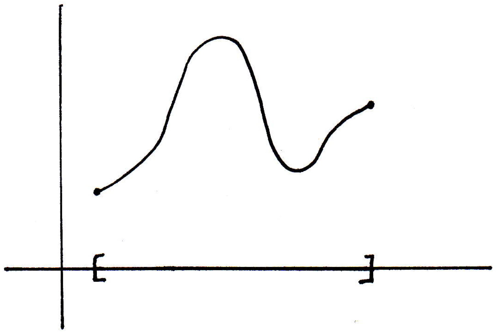
• A clearly not uniformly continuous function: Consider the following function:

  

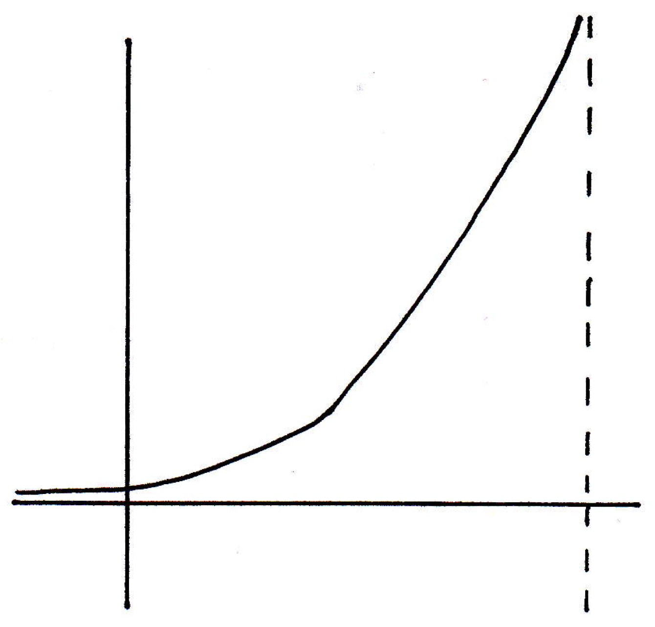
  Clearly this is not a uniformly continuous function. Why? Consider points $p$ and $q$ with a specified $\epsilon$-ball around $f(p)$ and another specified $\epsilon$-ball around $f(q)$:

  

  Then the $\delta$-ball that will land in the $\epsilon$-ball around $f(p)$ is actually quite large. But what does it take to land in the same $\epsilon$-ball around $f(q)$?

  

  Note: The $\epsilon$-balls in the picture are not actually the exact same size and should be redrawn. When they are redrawn, the $\delta$-ball around $q$ will still need to be much smaller than that around $p$ to ensure landing in the $\epsilon$-balls around $f(q)$ and $f(p)$.

  That by itself, by checking two points $p$ and $q$, and seeing that the $\delta$-balls were different, doesn't necessarily make the given function not uniformly continuous. Right? Because you might say well the $\delta$-ball around $q$ works for $p$ as well because it's smaller. But what's the difficulty? Will the $\delta$-ball around $q$ work for all points? No. Which ones are you going to worry about? The points beyond $q$ to the right. The $\delta$-ball around $q$ will no longer work because the function is doing something crazy. And why is it allowed to get away and do something crazy? Well, it's because the domain of the function was not closed to the right. If we had demanded that the function end at the vertical asymptote and be defined there, then this function could not have gone off to infinity and still be continuous. So we see in a very essential way the fact what uniform continuity is demanding of us. It's demanding the same $\delta$ work for every $\epsilon$. So what's the big deal here? When are functions going to be uniformly continuous?

• Theorem about continuous mapping with compact domain: Let $f\colon X\to Y$ be a continuous function, where $X$ is compact. Then $f$ is uniformly continuous on $X$.

  In the example given above, this theorem is pointing out where the problem is. It's bringing up the fact that if you had known the domain was compact, then we would have been in good shape. For example, if the domain had stopped right before it had gotten to the asymptote, then we'd still be okay. Why? What $\delta$ would work for every point? The $\delta$ that worked at the endpoint. That would work everywhere to the left. So this kind of gives a hint as to what is going on with the theorem.

  Now, why is the theorem above so important? Why do we care so much about uniform continuity? Well, uniform continuity basically says the same $\delta$ works for every $\epsilon$. It just means that for any target distance you name, I can tell you how close you have to be to land within $\epsilon$. The upshot of it all is that it doesn't matter where you are. That's the important part. And the above theorem is saying that you have uniform continuity whenever you have continuity on a compact set.

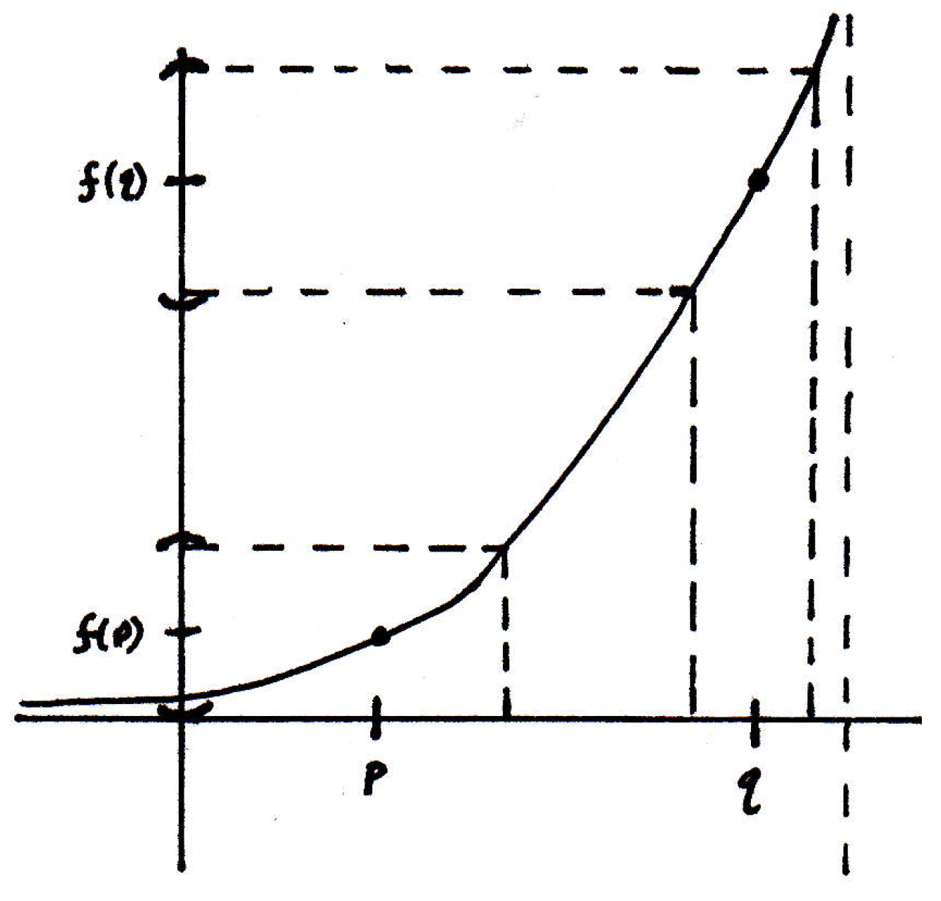
• Proof of theorem above (idea): Let's see if we can develop some intuition as to why the theorem above is true. How is compactness going to help us here? Let's draw another picture, where we start with a compact set (note that the $X$ used in this intuition-developing example need not be a subset of the real line; it could be a subset of any metric space; it could be one-dimensional, two-dimensional, infinite dimensional, etc.):

  

  So above is a compact set in the real line, and we have a function that's defined on it that's continuous:

  

  What $\delta$ is going to work for every $\epsilon$? So maybe we consider points $p$ and $q$ again:

  

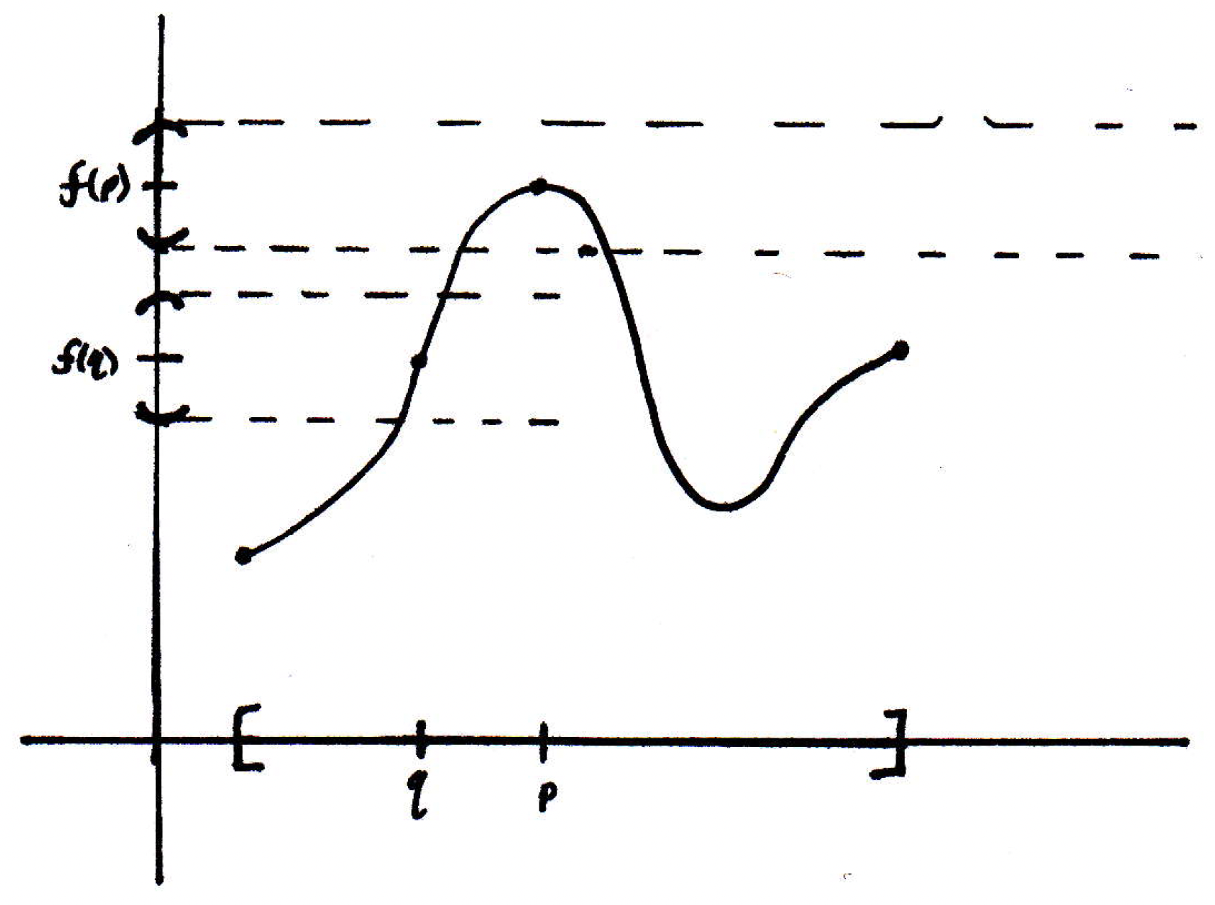
  The $\epsilon$-balls around $f(p)$ and $f(q)$ are the same, but the requisite $\delta$-balls around $p$ and $q$ are obviously different. (The $\delta$-ball around $q$ would have to be much smaller than the $\delta$-ball around $p$ to ensure that the images are within $\epsilon$ of the curve $f$.) We could go over a few places and find some $\delta$-balls that would keep things within $\epsilon$ as well. So lots of different $\delta$'s. What $\delta$ is going to work for every given $\epsilon$? The smallest one! Is there a smallest one? Not necessarily. There wasn't a smallest one in the previous example. (The $\delta$-balls got smaller and smaller as we went to the right. How do we know the $\delta$-balls in the current examples won't get smaller and smaller and smaller? What about the point at which the slope is greatest? Intuition is good there, but we have to be a little bit careful. If the function had a derivative, which we have not defined yet, and which also the function may not actually have (the only requirement is that it be continuous but not necessarily differentiable), but if we could talk about slopes, then it would certainly make sense perhaps to think that where the slope was greatest the requisite $\delta$-ball would be smallest. Even this idea presents a slight problem; for example, $\sqrt[3]{x}$ has an infinite slope at the origin, and the idea of a "maximal slope" is a problematic notion. But it is a good intuition that somehow slope is related to this notion of closeness and everything.

• Proof of theorem (book's idea): There many ways to prove the theorem in question. We'll give another one here than that from the book, but here's the idea from the book. Every point in the compact set has a $\delta$-ball associated with it. Those $\delta$-balls form an open cover of the open set which is compact; therefore, there is a finite subcover of the set. And the $\delta$-balls don't necessarily guarantee anything. You have to be careful. And so the book starts off with balls bigger than you need and works out some nifty metric arguments to make everything work. It's worth reading and understanding, but we'll present a different proof that appeals to a famous lemma which we will also prove.

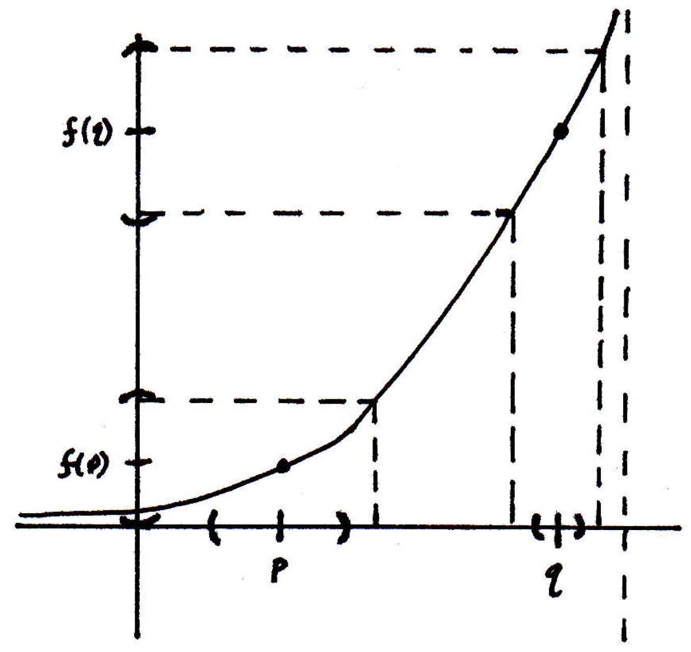
• Proof of theorem: Given $\epsilon>0$. [Our goal is to find a $\delta>0$ that will work for all points $p$.] Each point $x\in X$ has a $\delta$-ball, and we'll call this a $\delta_x$-ball because this ball may depend on $x$, that satisfies the condition for continuity, namely that $d(y,x)<\delta_x\implies d(f(y),f(x))<\eta$, where we will treat $\eta$ as a placeholder for now because we will see later what $\eta$ needs to be in order for our proof to work. You name a $\eta$ and we can make this true for a particular $\delta_x$ that may depend on $x$. We'll see momentarily what $\eta$ should be.

  The $\delta$-balls cover $X$:

  

  Here's a question: Would we be done if our argument if we could show that for a small enough distance that if you give me two points that are close enough anytime we thrown them down randomly in the picture above that they lie in one interval? Ought that be true? Is that necessarily true? (If we could answer this question, then we would be done as we will see momentarily.) That is, can we find a $\delta$ such that if $d(p,q)<\delta$ then $p$ and $q$ are in the same element of the cover set (i.e., if $p$ and $q$ are in the same element, namely a cover set, from the open cover set as a whole)? Consider the following picture where you're given $p$ and $q$:

  

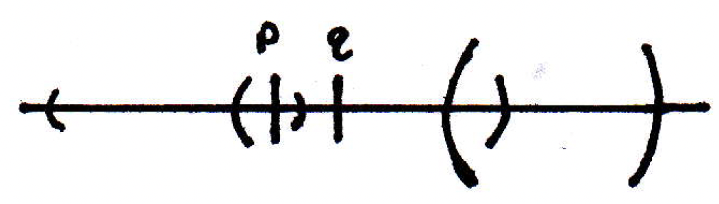
  Do they not both lie in one element of the cover set, namely the interval with medium-sized parentheses? If you could do that, then we could bound the distance between $p$ and $q$ by their distance to the center point $x$ of this cover:

  

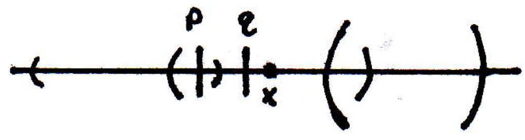
  If so, then we have that

  $$d(f(p),f(q))\leq d(f(p),f(x))+d(f(x),f(q))<\eta+\eta$$

  since $d(p,x)<\delta_x$ and $d(q,x)<\delta_x$ (because they were in the same ball). If we want $\eta+\eta<\epsilon$, then we need to make $\eta=\frac{\epsilon}{2}$. So that's the choice we should make at the beginning for $\eta$.

  What do we have here? If I could find a $\delta$ that's small enough so that anytime two things $p$ and $q$ are within $\delta$ of each other they live in the same element of the cover set, then certainly they are within $\delta_x$ of each other. That's what the cover is that is explicitly drawn above. It is a $\delta_x$-ball.

  Is the whole conjecture from above true? Yes. It's such an important fact that it has its own name. It's called the Lebesgue covering lemma. It's an excuse to prove something that is not covered in Rudin but is used very very often in many contexts.

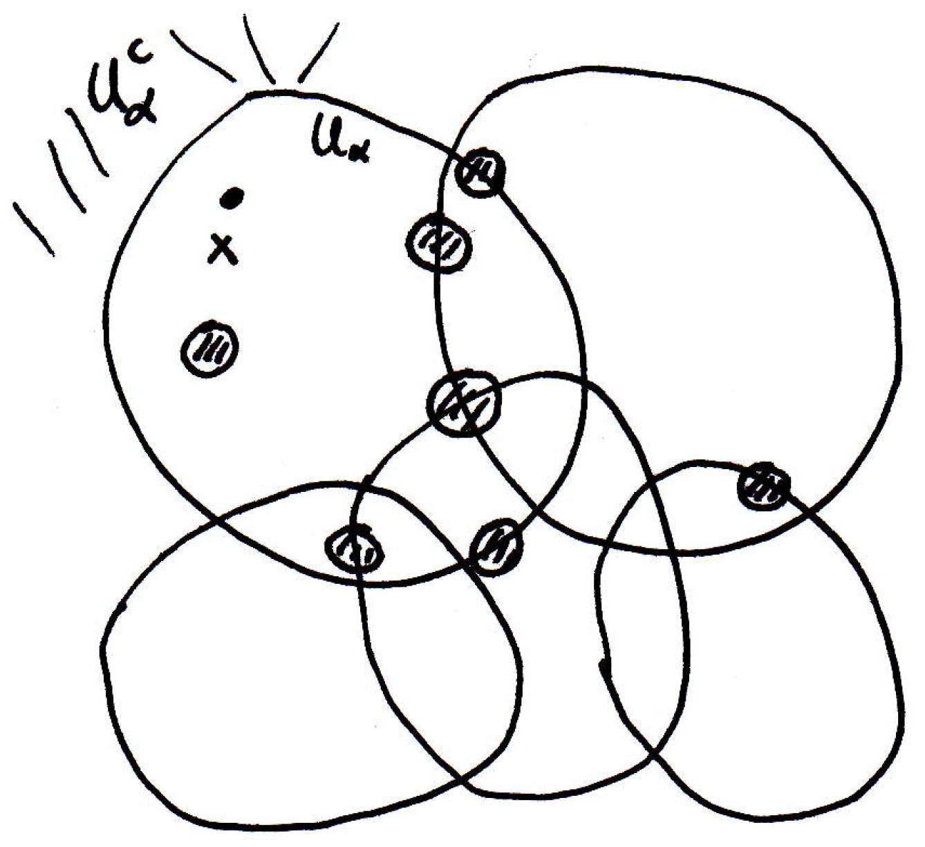
• Lebesgue covering theorem: If $\{U_\alpha\}$ is an open cover of a compact metric space $X$, then there exists $\delta>0$ such that for all $x\in X$, $B_\delta(x)$ is contained in some $U_\alpha$.

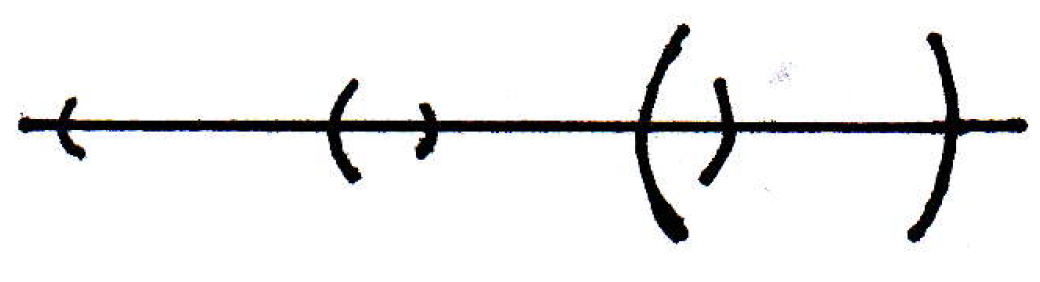
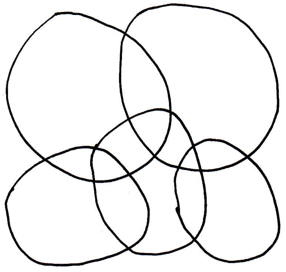
  The $\delta$ referenced above has a special name. It's called the Lebesgue number of the cover. This Lebesgue number will exist and be bigger than 0 if the space $X$ is compact. The picture you should have in your head is something like the following where the space $X$ is covered by a bunch of sets like so:

  

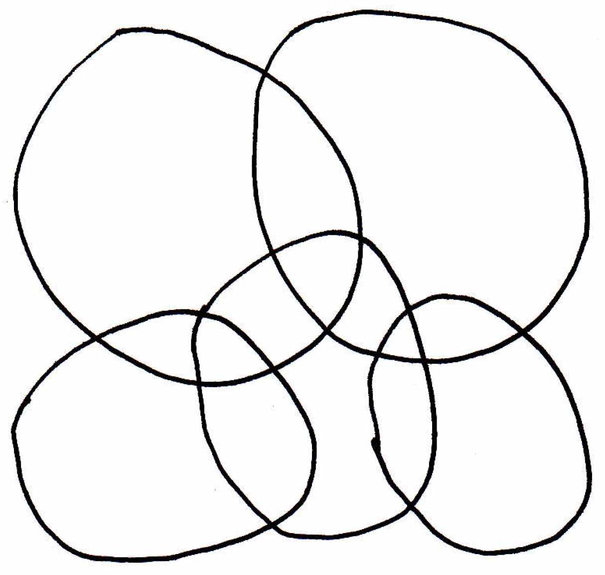
  The Lebesgue number is basically a number $\delta$ such that you give me a little pancake of radius $\delta$, and if I throw that pancake anywhere in the picture, it will land completely within one of the sets (i.e., within one of the covering sets). If there is such a number $\delta$, then it's called the Lebesgue number, and the claim is that if the space $X$ is compact, then there will exist such a number. In the picture above, we might have something like the following:

  

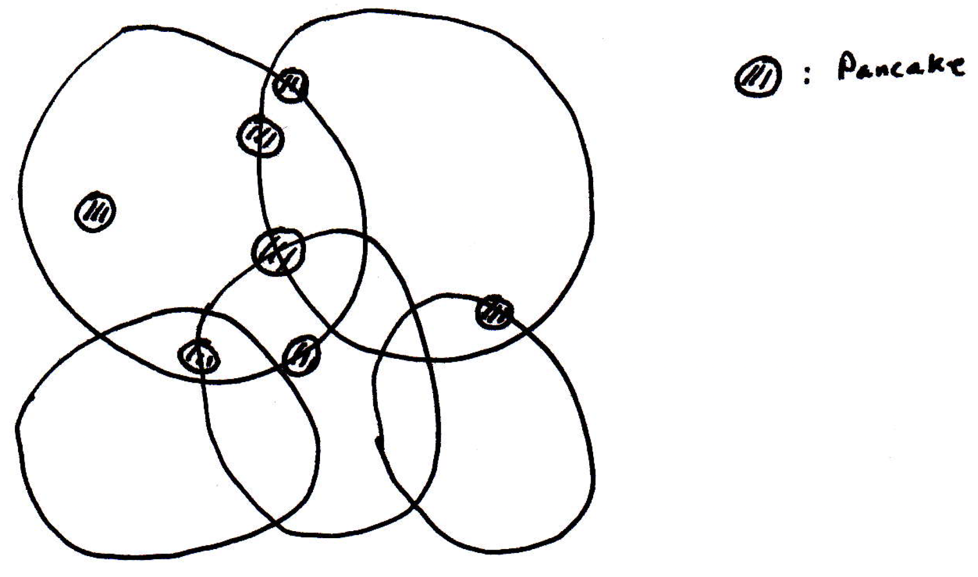
  That is, we have a pancake of about the given size in the picture and no matter where we put it, it will lie completely in one element of the cover. Now, this would not necessarily be true if the space were not compact. Imagine the following space, the open interval where it were covered like so:

  

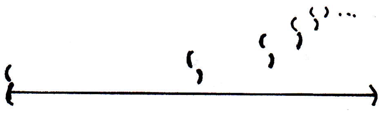
  So the open interval is covered by many open sets that get smaller and smaller as you go to the right. Throw a pancake down of any size and you get into trouble as you go to the right. So the lemma does not hold if the space is not compact. And that is what we were basically saying before the statement of the lemma here.

  If there's a pancake that you can throw down so that it lands completely within one of those $\delta_x$-balls, that's the $\delta$ that we're interested in, then we're in good shape because we'll be able to complete the proof as desired. So let's see why the Lebesgue number exists.

• Lebesgue theorem (proof): How should we start here? The space is compact. Since $X$ is compact, there exists a finite subcover $\{U_{\alpha_i}\}_{i=1}^n$. So then what? We can remove all but finitely many of the balls shown above in the picture. That's nice.

  If the covering sets of our compact space are open, then their complements are closed. Suppose we have a point $x$ in some $U_\alpha$:

  

  Then all the space outside of $U_\alpha$, which is its complement $U_\alpha^c$, is closed. Then it should make sense to talk about defining a distance between $x$ and $U_\alpha^c$ since $U_\alpha^c$ is closed.

  How should such a distance be defined? If a set $K$ is closed, then we can define $d(x,K)=\inf\{d(x,y) : y\in K\}=\inf_{y\in K} d(,x,y)$. What can we say about this distance notion? We claim that $d(x,K)$ is a continuous function of $x$. Basically use triangle inequality and compare $x$ to some other close point $y$. So then what?

  If the pictured sets cover $X$, then $x$ is an at least one of the covering sets. And so the distance between $x$ and the complement of the covering that $x$ is in is going to be nonzero. Now, if $x$ is not in a covering set, then the distance between $x$ and the complement of the set that $x$ is not in will be 0. So we only have finitely many covering sets. Let's look at the distance between $x$ and all of the complements of the covering sets. What would it mean if we found a Lebesgue number? What would that mean? If we could throw pancakes down in our original picture and have them land in a set, then that's really saying that the distance from $x$ to one of the complements is bigger than $\delta$. So if we could show that for at least one of the sets that there is a $\delta$-ball around a point $x$ that separates it from a complement by a minimum distance $\delta$. Then we should be in good shop. So let's look at all distances between $x$ and the complement of the covering set that $x$ is in. So let's look at $d(x,U_{\alpha_i}^c)$. There's one for every $i$. Now, we're hoping to show that the minimum of all the $d(x,U_{\alpha_i}^c)$ is bigger than 0 for every $x$. We could add up all the distances and divide by $n$ (so taking the average) to get a function of $x$:

  $$f(x)=\frac{1}{n}\sum_{i=1}^n d(x,U_{\alpha_i}^c).$$

  What can we say about the function $f$ that is the average distance from $x$ to the complements? It must be continuous because it's the sum of continuous functions. What else? It's defined on a compact set. So it's a continuous function on a compact set. Thus, by a theorem we discussed recently, it must attain its maximum and minimum. What are we concerned worth? The minimum value. So $f$ attains its minimum value. Let's call it $\delta$. What would it mean for the average of a bunch of distance to be at least $\delta$? It would mean one of them is at least $\delta$. And that's all we need. And that's the set that the pancake falls in. So if $f(x)\geq\delta$, then at least one of $d(x,U_{\alpha_i}^c)\geq\delta$, so for this $i$, we have $B_\delta(x)\subset U_i$.

  For the above, why is $\delta>0$? The fact that

  

  is a cover means that for every $x$ it's in one of the covering sets. Thus, our function $f$ has to be nonzero everywhere. So its minimum value has to be bigger than 0. That is, $\delta>0$ because $f(x)>0$ at each $x$ since the $\{U_{\alpha_i}\}$ are a cover, and note here that we are really using the fact that $f$ attains its minimum value because you may worry that even if $f(x)>0$ then its infimum may be 0, but the infimum cannot be zero here because $f$ achieves its minimum somewhere, and that minimum is bigger than 0.

Connectedness and its relation to continuity

How is connectedness related to continuity?

• Continuity preserves: We've seen that continuity preserves lots of different things. Continuity preserves limits. It preserves compactness. (The image of a compact set is compact.) Continuity also preserves connected sets. So if you take the image of a connected set, then the image is connected.

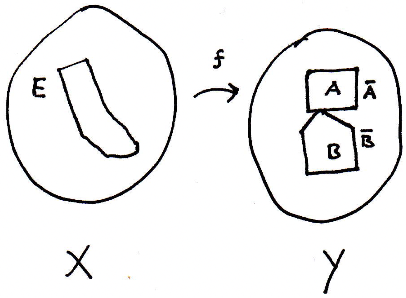
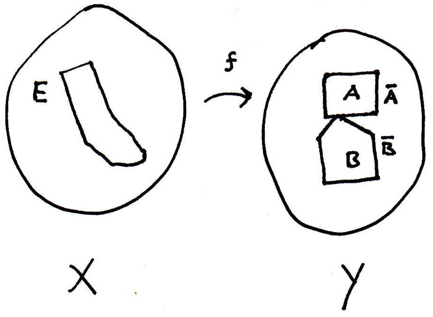
• Theorem concerning images of connected sets being connected: If $f\colon X\to Y$ is continuous, and $E$ is a connected subset of $X$, then $f(E)$ is connected.

  This is a very believable result. You cannot continuously deform a connected set into something that is not connected without introducing a discontinuity. How should we prove this? Let's draw a picture:

  

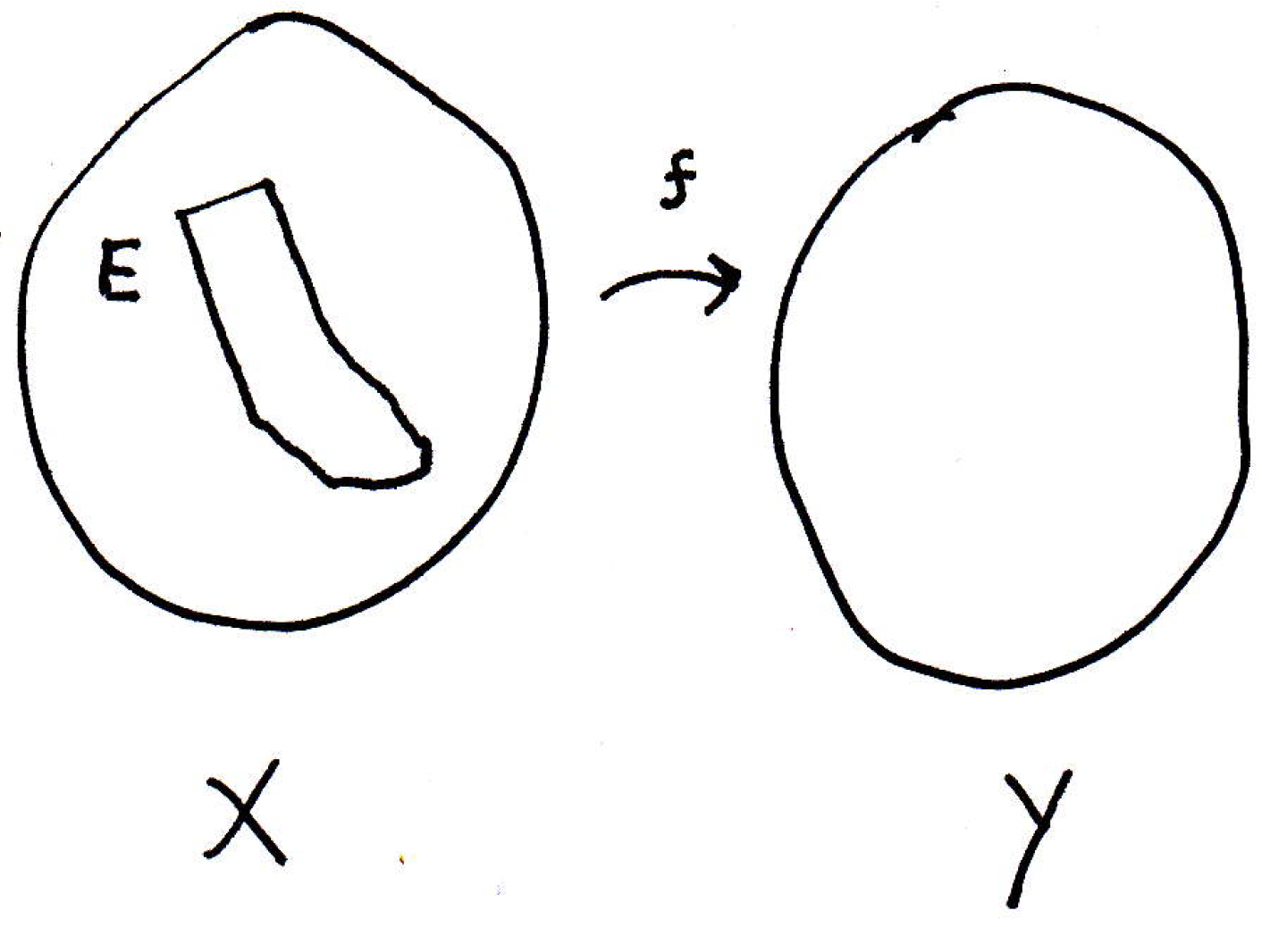
  The claim is the image, $f(E)$, is connected. So what's the perfect way to start off this proof? What does it mean for a set to be connected? It cannot be separated. Not the union of two nonempty, separated sets. It's always easier to work with sets that are not connected so if we want to show the image is connected, then maybe we should construct a proof by contraposition.

  Suppose $f(E)$ is not connected. Then $f(E)$ is separated (our goal will be to show that $E$ is separated and therefore not connected); that is, $f(E)=A\cup B$, where $A$ and $B$ are separated sets (which means $A$ and $B$ are nonempty, and we have $\overline{A}\cap B=A\cap\overline{B}=\emptyset$). Let's draw a picture that cannot be true:

  

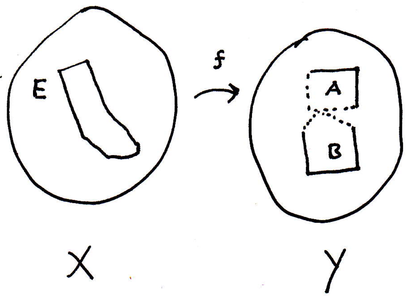
  Now, $f$ is continuous, and that means all sorts of different things. Now, if $A$ and $B$ were both open sets, then we would have an easy proof on our hands. If $A$ is open, then because $f$ is continuous, the preimage of $A$ is open. The same goes for $B$. So we would have the union of two open sets. In $E$ the sets are clopen.

  We can look at the closures of $A$ and $B$; that is, we'll look at $\overline{A}$ and $\overline{B}$:

  

  Now, what do we know about $\overline{A}$ and $\overline{B}$? They are both closed of course, but because $f(E)$ is separated, we must have $\overline{A}\cap B=\emptyset$ and $A\cap\overline{B}=\emptyset$. It might be the case that $\overline{A}\cap\overline{B}\neq\emptyset$. (This is reflected in the picture.) What's the next thing we should do? We don't really know anything about $A$ and $B$. They're not necessarily open or closed. If they're open, then we could take their inverse images and they would be open. If they were closed, then their inverse images would be closed. So let's take the inverse images of $\overline{A}$ and $\overline{B}$. What do we know about those? They're closed. Let's denote these preimages as follows:

  $$K_A=f^{-1}(\overline{A}) \qquad\text{and}\qquad K_B=f^{-1}(\overline{B}).$$

  Both $K_A$ and $K_B$ are closed since $f$ is continuous, and they are sitting somewhere in $X$, and maybe they look as follows:

  

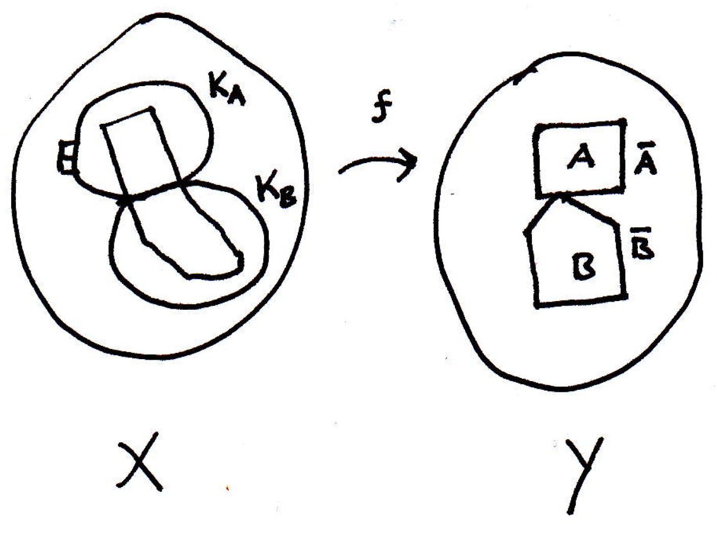
  What can we say here? What we want to do is use these sets somehow to produce a separation of $E$, which would give us the completion of the proof by contraposition. So what's the separation that might be suggested? What could be a good proposal for a separation of $E$? We know $K_A$ and $K_B$ could not quite work because they might intersect (because $\overline{A}$ and $\overline{B}$ might intersect so their inverse images would intersect) as shown in the picture. What about the interiors? We might be in trouble because we might leave out some points right at the boundary. What about $f^{-1}(A)$ and $f^{-1}(B)$? These are smaller sets. Let's let

  $$E_1=f^{-1}(A)\cap E \qquad\text{and}\qquad E_2=f^{-1}(B)\cap E,$$

  where we are intersecting $f^{-1}(A)$ and $f^{-1}(B)$ with $E$ because these inverse images may contain many other points in $X$. Now let's update our picture to reflect this:

  

  Then clearly $E_1$ and $E_2$ are disjoint because $A$ and $B$ are disjoint. So inverse images are disjoint. Are $E_1$ and $E_2$ nonempty? Yes. Why? Because $A$ and $B$ are nonempty. We hope to show $E_1$ and $E_2$ are a separation; that is, we want to show that the closure of $E_1$ does not have a nonempty intersection with $E_2$ and vice-versa. So our claim is that $E_1$ and $E_2$ separate $E$. Let's see why.

  Well, $E_1\subset K_A$, which is closed. (We know that $E_1\subset K_A$ since $f^{-1}(A)\subset f^{-1}(\overline{A})$.) Similarly, $E_2\subset K_B$, which is also closed. Can we justify that the closure of $E_1$ does not contain a point of $E_2$; that is, can we show that $\overline{E_1}\cap E_2=\emptyset$? Note that $\overline{E_1}$ is the smallest closed set containing $E_1$; since $K_A$ is closed and contains $E_1$ it must also be the case that $\overline{E_1}\subset K_A$. Similarly, $\overline{E_2}\subset K_B$. Again, why is it the case that $\overline{E_1}\cap E_2=\emptyset$? Well, $E_1$ is in $K_A$, and we claimed that $K_A$ does not intersect $E_2$; that is $K_A\cap E_2=\emptyset$. Why? We have $K_A=f^{-1}(\overline{A})$, but $\overline{A}$ is disjoint from $B$, and $E_2$ is contained in the inverse image of $B$, and $\overline{A}\cap B=\emptyset$. That is, we have that $K_A\cap E_2=\emptyset$ because $f^{-1}(\overline{A})=K_A$ and $f^{-1}(B)=E_2$, and we also have that $\overline{A}\cap B=\emptyset$. So we've used the separation property here. And similarly you can show that $K_B\cap E_1=\emptyset$. Therefore we have a separation. So $E$ is separated. And this concludes the proof by contraposition. So the image of connected sets is connected. No big surprise there, but it gives a very useful consequence.

• Intermediate value theorem (ideas): Can we see why this theorem is about dealing with images of connected sets? What does the intermediate value theorem say? It says that if $f\colon[a,b]\to\R$ is continuous, and $f(a)<c<f(b)$, then there exists $x\in(a,b)$ such that $f(x)=c$.

  A classic picture of this situation is the following:

  

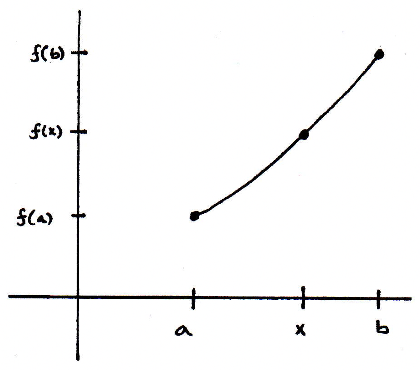
  Why is this a consequence of the theorem about connected sets? Well, we have a connected interval $[a,b]$. Its image is connected. Suppose the image never hits $f(x)=c$, but it hits $f(a)$ and $f(b)$. Then the image would be disconnected. In fact, you could disconnect it using the part below $f(x)=c$ and the part above $f(x)=c$. We claim that's a disconnection because the closure of a part above $f(x)=c$ can at most contain $f(x)=c$. It can't intersect the other part. And vice-versa.

• Intermediate value theorem (proof): The fact that $[a,b]$ is connected implies that the image $f([a,b])$ is connected, but if $f(x)=c$ is not achieved, then $c$ would disconnect $f([a,b])$. That's the basic idea. More formally, we would look at $(c,+\infty)\cap f([a,b])$ and $(-\infty,c)\cap f([a,b])$ which forms a separation. That's the basic idea.

• Converse of intermediate value theorem: Is the converse of the intermediate value theorem true? That is, if a function has an intermediate value property, must it be continuous? No. Consider the function

  $$f(x)= \begin{cases} 0 & \text{if}\ x=0,\\ \sin(1/x) & \text{if}\ x\neq0. \end{cases}$$

  The graph basically looks like the following:

  

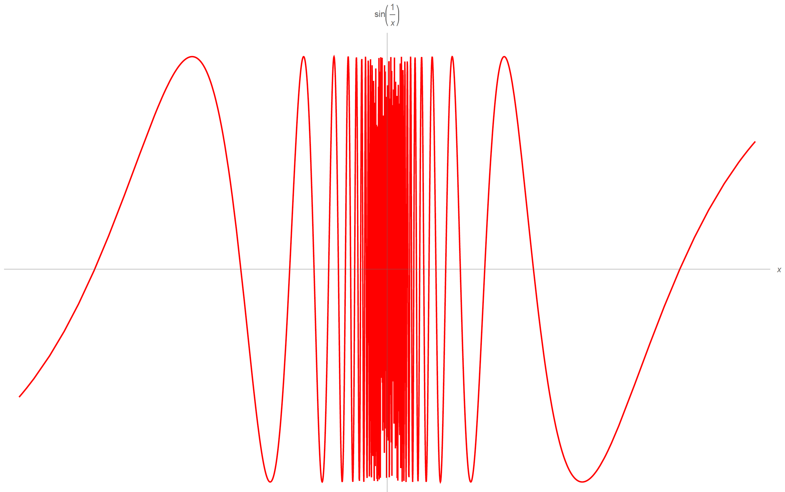
  The claim is that the function above is not continuous at 0, but it satisfies an intermediate value property.

• Next time (discontinuities): We know what it means for a function to be continuous everywhere. Is it possible for a function to be discontinuous everywhere? That's an interesting question. We'll explore it more next time.