24 - The derivative and Mean Value Theorem

The derivative and its relation to our work thus far

What is the derivative and how does it relate to what all we have developed thus far?

• Prelude: Much of the machinery we have been building up in this course has been heading towards being able to understand the concepts of calculus with attention to being very rigorous about some of the definitions. So let's define the derivative. We want to understand the derivatives, what it is and what it means. We have talked a good bit about continuous functions, and now we're interested in understanding when functions are what are called differentiable. So let's make a definition.

• Derivative (definition): A function $f\colon[a,b]\to\R$ is differentiable at $x\in[a,b]$ if the following limit exists:

  $$f'(x)=\lim_{t\to x}\frac{f(t)-f(x)}{t-x},$$

  where $t\in(a,b)$ but $t\neq x$.

• Remarks: The above definition probably looks very familiar. However, it often may be written slightly different in some textbooks, namely something like

  $$\lim_{h\to0}\frac{f(x+h)-f(x)}{h}.$$

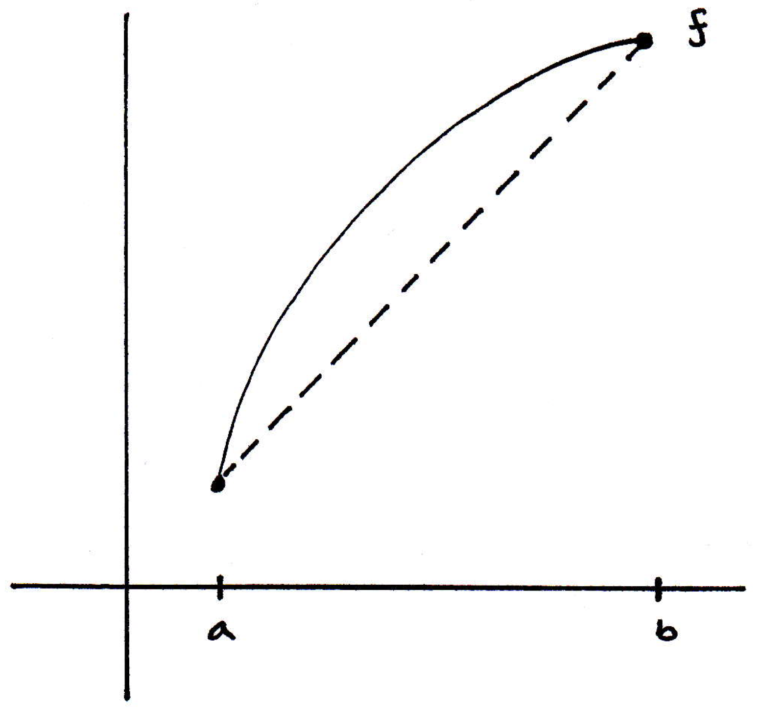
  The picture you might have in mind is something like the following:

  

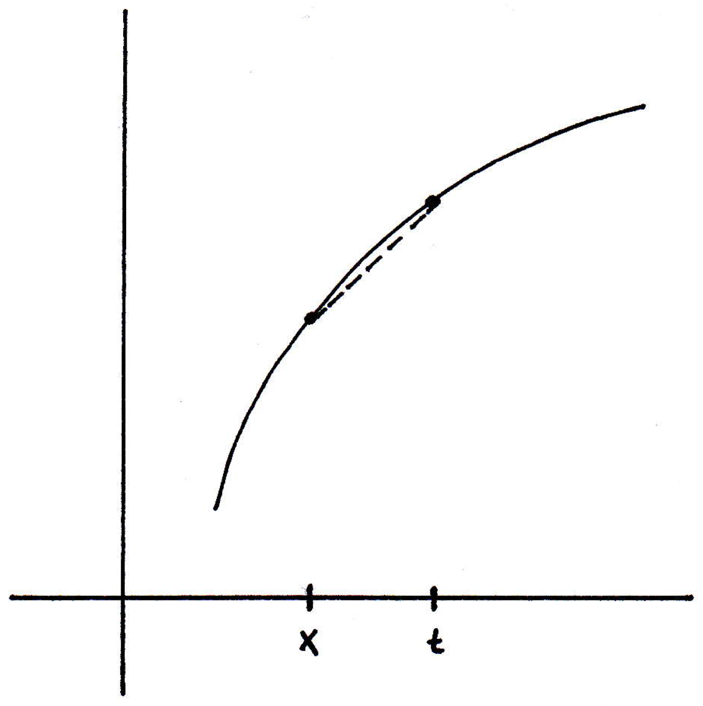
  So we have the graph of some function $f$, and we want to understand what's happening at a particular point $x$ and compare that to what's happening nearby at some point $t$ (or $x+h$ if we used the other commonly seen definition of the derivative). If we compared what's happening, then $f(t)-f(x)$ is basically the difference in the height of the graph of the function while $t-x$ is the length of the interval between $t$ and $x$. So $\frac{f(t)-f(x)}{t-x}$ is the "rise over the run" so you may think of it as the slope of the secant line connecting $f(x)$ and $f(t)$, as demonstrated in the figure above with the dashed line representing this secant line. And now what we do with the limit $\lim_{t\to x}\frac{f(t)-f(x)}{t-x}$ is we look at the slope of the secant line as we let $t$ get closer and closer to $x$. So we essentially have the following:

  $$f'(x)=\underbrace{\lim_{t\to x}\underbrace{\frac{f(t)-f(x)}{t-x}}_{\substack{\text{slopes of}\\\text{secant lines}}}}_{\substack{\text{limit of the slopes}\\\text{of the secant lines}}}.$$

  If that limit exists, then it appears that the slopes of the secant lines seem to converge, at least in this particular converge. So if we have a limit, then it is basically going to communicate the following: If we could place a secant line right at $x$, that is it subtended the points right at $x$ and a point very close nearby, then you'd get the slope of the following line, which we often call the tangent line:

  

  This line has slope $f'(x)$. That's the idea. Now, of course, we could let $t$ approach $x$ from the left, but the slopes would also converge.

• A non-differentiable function: The example above is to be contrasted with another example where we can run into a problem. Consider the following function:

  

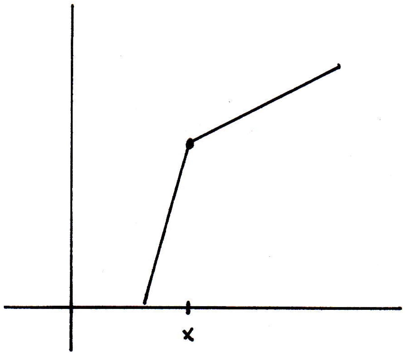
  Certainly this function is continuous at $x$, but what happens if we look at the slopes of the secant lines? If you look at any secant on the right-hand side of $x$, then because that line is straight you just get the slope of the line segment as the slope of the secant line. Take the limit from the right, then that limit from the right exists and it converges to the slope of the line segment. The limit from the left exists for the same reason, and it converges to a different slope. So does the limit exist? No. So the function is not differentiable at $x$.

• Some questions: Let's see if we can get a feel for how some questions should turn out to be:

  • Continuity implies differentiability (?): If $f$ is continuous on $[a,b]$, then is $f$ differentiable on $[a,b]$? No. The example above shows this is not necessarily the case.
  • Differentiability implies continuity (?): If $f$ is differentiable on $[a,b]$, then must $f$ be continuous on $[a,b]$? Yes, how do we prove this? It's not too hard if we know properties of limits. When we take the limit of a function, we know that the limit of a product is the product of the limits.

• Differentiability implies continuity: If we want to verify that $f$ is continuous, then it should suffice to show that if $t\to x$, then

  $$\lim_{t\to x} f(t)-f(x)=0=\lim_{t\to x}\frac{f(t)-f(x)}{x-a}\cdot(t-x)=f'(x)\cdot0=0.$$

  So we've just verified that $\lim_{t\to x}f(t)=f(x)$, which is what it means to be continuous. So differentiable functions are continuous.

• Differentiability implying continuity over an interval: If $f$ is differentiable on $[a,b]$, then must $f'$ be continuous? It's clear that $f'$ must exist since $f$ is differentiable on $[a,b]$, but must this function $f'$ be continuous? Consider the following function:

  $$f(x)= \begin{cases} x^{4/3}\sin(1/x) & \text{if}\ x\neq0,\\ 0 & \text{if}\ x=0. \end{cases}$$

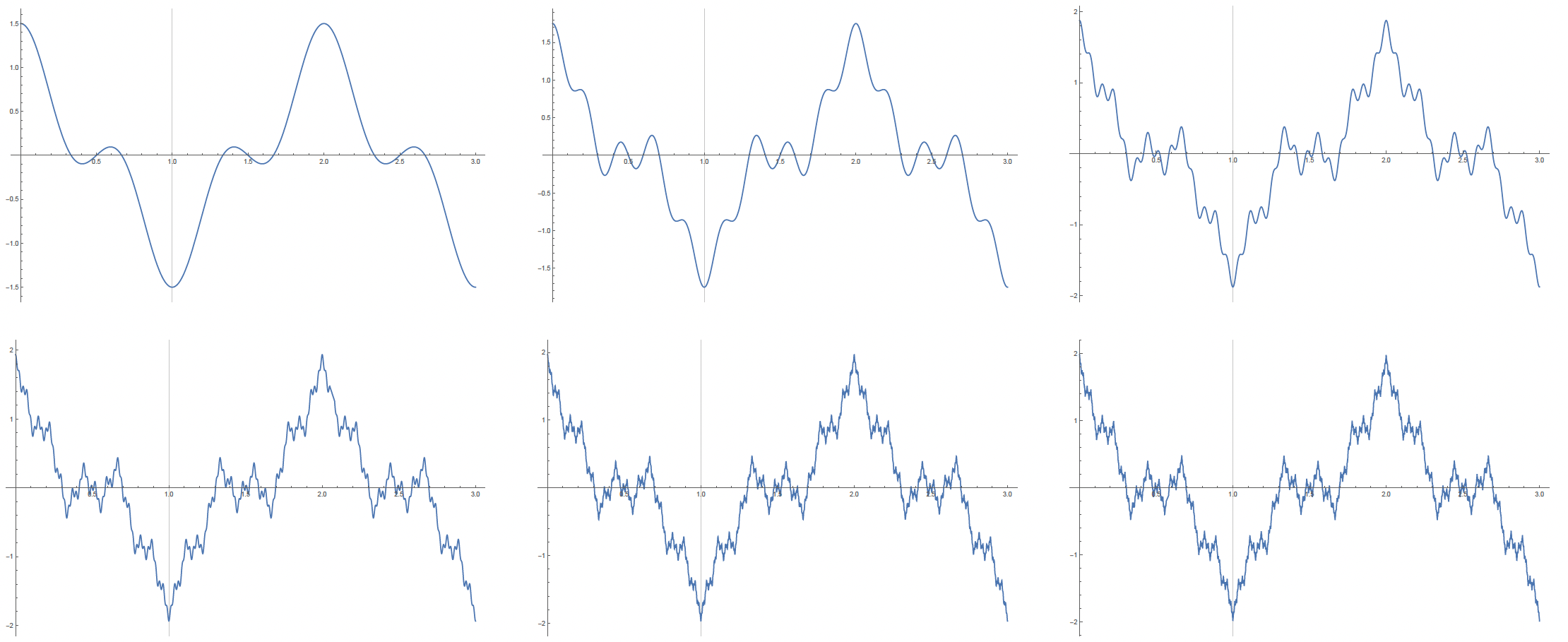
  This function will oscillate more and more as $x$ gets closer and closer to 0. But now we are multiplying $\sin(1/x)$ by $x^{4/3}$ so this function will have an amplitude that is governed by the curve $y=\pm x^{4/3}$. The graphs below show what this function looks like for domains $[-0.1,0.1]$, $[-1,1]$, and $[-10,10]$, respectively, where the curves $y=\pm x^{4/3}$ have also been graphed in blue to show the bounding behavior:

  

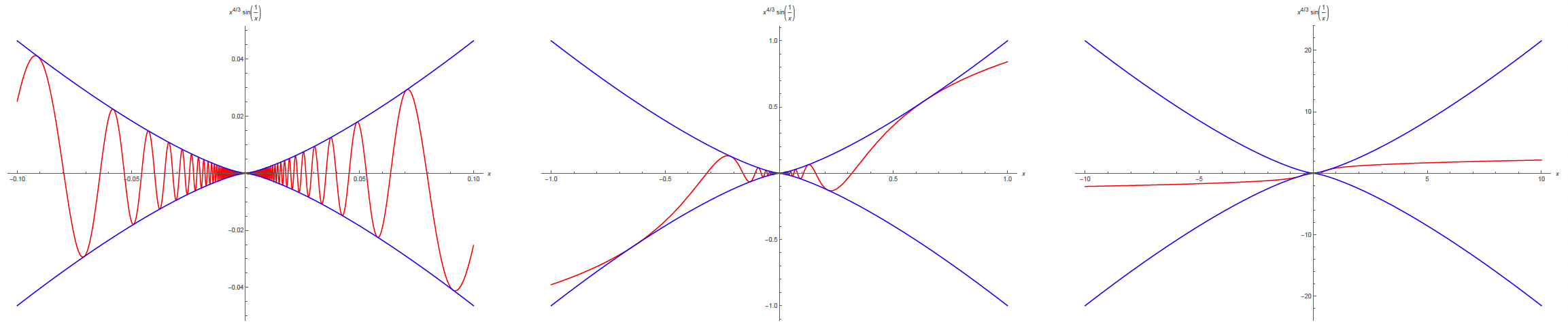
  Is $f$ differentiable? Yes. Why? Well, away from 0 it's clearly differentiable, but where's the only place you might worry whether or not it's differentiable. Why, if we start looking at secant lines, with one end at 0, and the other end somewhere else, why this thing will actually have a limiting slope, the secant line. The sort of "envelope functions" (i.e., $y=\pm x^{4/3}$) will start squeezing the secant lines, wherever you start putting them, enough so that if you blow the picture up then it will look more and more linear.

  If we take the derivative, using results from calculus just to see what happens, then we end up with the following graphs for $f'$, where these graphs are made on the corresponding domains as those above:

  

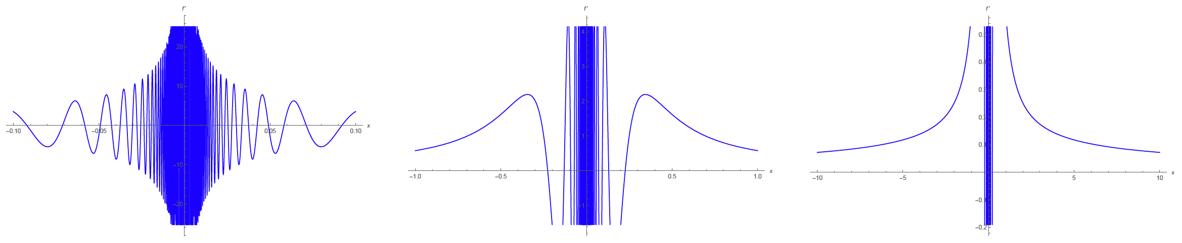
  What we find here is that $f$ has a derivative everywhere, but the derivative function is not continuous. The reason we chose $\frac{4}{3}$ in the expression for the variable amplitude (i.e., in $x^{4/3}\sin(1/x)$) was because if the power of $x$ happened to be less than 1, then we'd be in trouble in regards to trying to make $f$ differentiable. So it has to be bigger than 1 to make $f$ differentiable. And the power has to be less than 2 to get the derivative to blow up towards the origin. (It just needs to be a number between 1 and 2. There's nothing special about $\frac{4}{3}$.)

  So we return to our question: If $f$ is differentiable on $[a,b]$, then must $f'$ be continuous? No, as the example above illustrates. Even though the answer is no, and we see that $f'$ is not always continuous, it is true that $f'$ always satisfies an intermediate value property. Not only that, but we can also say that $f'$ has no simple discontinuities; that is, if $f'$ does have any discontinuities, then they are of the second kind.

• Derivatives that are continuous: Given the result established above, namely that the derivative of a differentiable function on $[a,b]$ need not be continuous, it makes sense that we would have a name for functions whose derivatives are continuous, since this is not always the case.

  We call a function $f$ a $C^1$-function if $f'$ exists and is continuous. So the above example is an example of a function that is not a $C^1$-function. Similarly, we will call a function a $C^k$-function if the $k$th derivative $f^{(k)}$ exists and is continuous. We might ask ourselves whether or not there are functions that are $C^1$ but not $C^2$. Or functions that are $C^2$ but not $C^3$. Probably because we have names for these functions! But how might we construct such functions? Consider the function

  $$f(x)= \begin{cases} x^p\sin(1/x) & \text{if}\ x\neq0,\\ 0 & \text{if}\ x=0. \end{cases}$$

  Then $f$ is a $C^0$-function (but not $C^1$) if $p\in(1,2)$. If $p\in(2,3)$, then we'll get functions that are $C^1$ but not $C^2$, and so on. So you can construct whole classes of these things. We should note that $C^0$ represents continuous functions. If you take derivatives many many times and if all the derivatives exist, then we have a special name. Those are called $C^\infty$-functions. And $C^\infty$-functions are actually called "smooth" functions. So the word "smooth" in analysis has a technical meaning. It means all the derivatives exist and are continuous.

  The following more precise definition from here may help:

  $\bm{C^\infty}$-functions. A function with $k$ continuous derivatives is called a $C^k$-function. In order to specify a $C^k$-function on a domain $X$, the notation $C^k(X)$ is used. The most common $C^k$ space is $C^0$, the space of continuous functions, whereas $C^1$ is the space of continuously differentiable functions. Of course, any smooth function is $C^k$, and when $\ell>k$, then any $C^\ell$-function is $C^k$. It is natural think of a $C^k$-function as being a little bit rough, but the graph of a $C^3$ function "looks" smooth. Examples of $C^k$ functions are $|x|^{k+1}$ (for $k$ even) and $x^{k+1}\sin(1/x)$, which do not have a $(k+1)$st derivative at 0.

• Results concerning derivatives: Since $f'$ is a limit, then it follows from properties of limits of functions, namely the sum, difference, product, and quotient rules all follow for derivatives. So, for example, we claim that $(f+g)'=f'+g'$ because the limit of a sum is the sum of the limits. What about $(fg)'=f'g+fg'$? Where does this come from? We can let $h=fg$, and we can give a picture as motivation for the proof. Imagine $h$ is the size of a box whose height and width are given by $f$ and $g$. And as you increase the argument, which you might think of as time, the box is growing. So imagine at some time we have a box of height $f(x)$ and width $g(x)$:

  

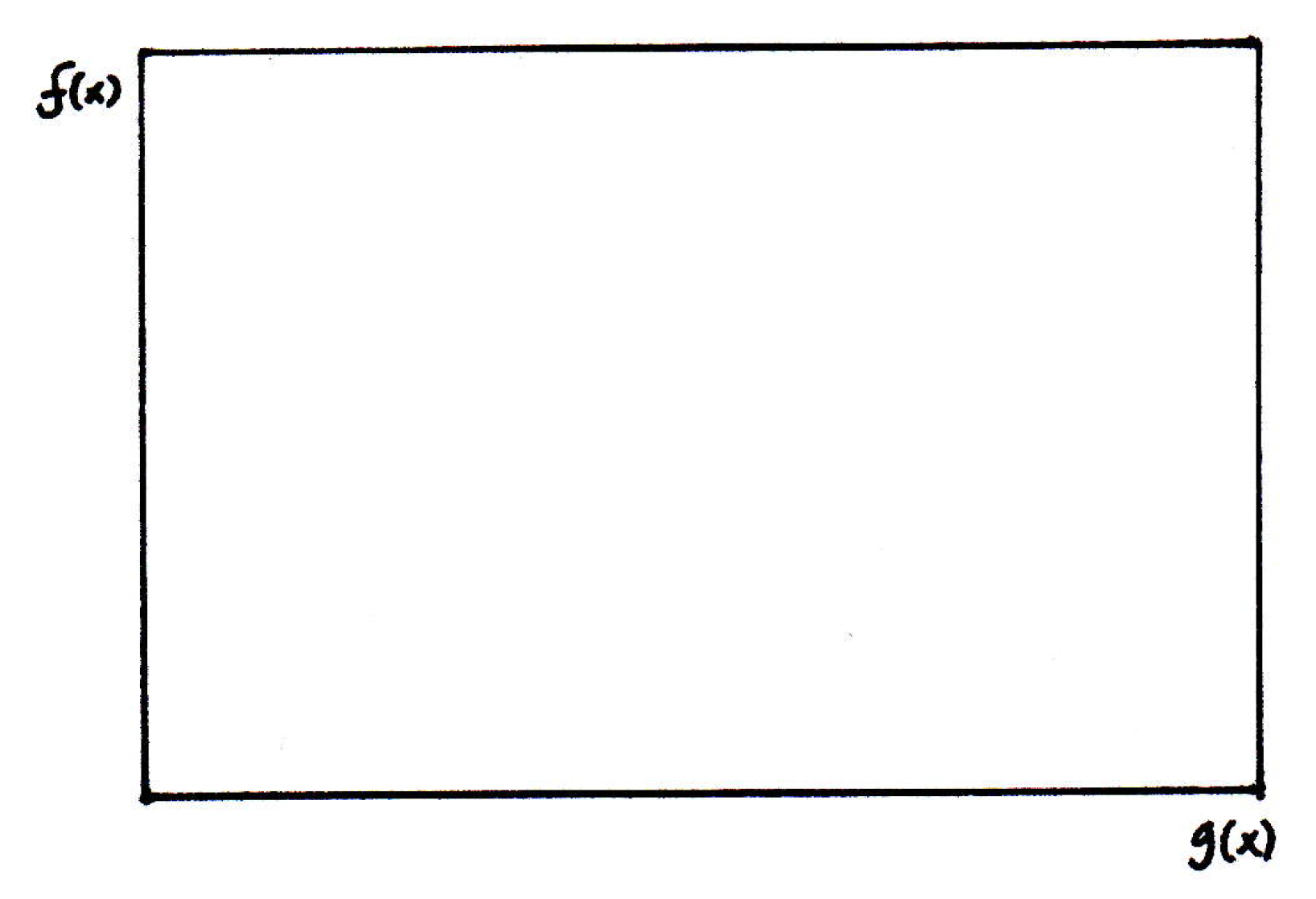
  But then sometime a little later on, the height is now $f(t)$ and the width is $g(t)$:

  

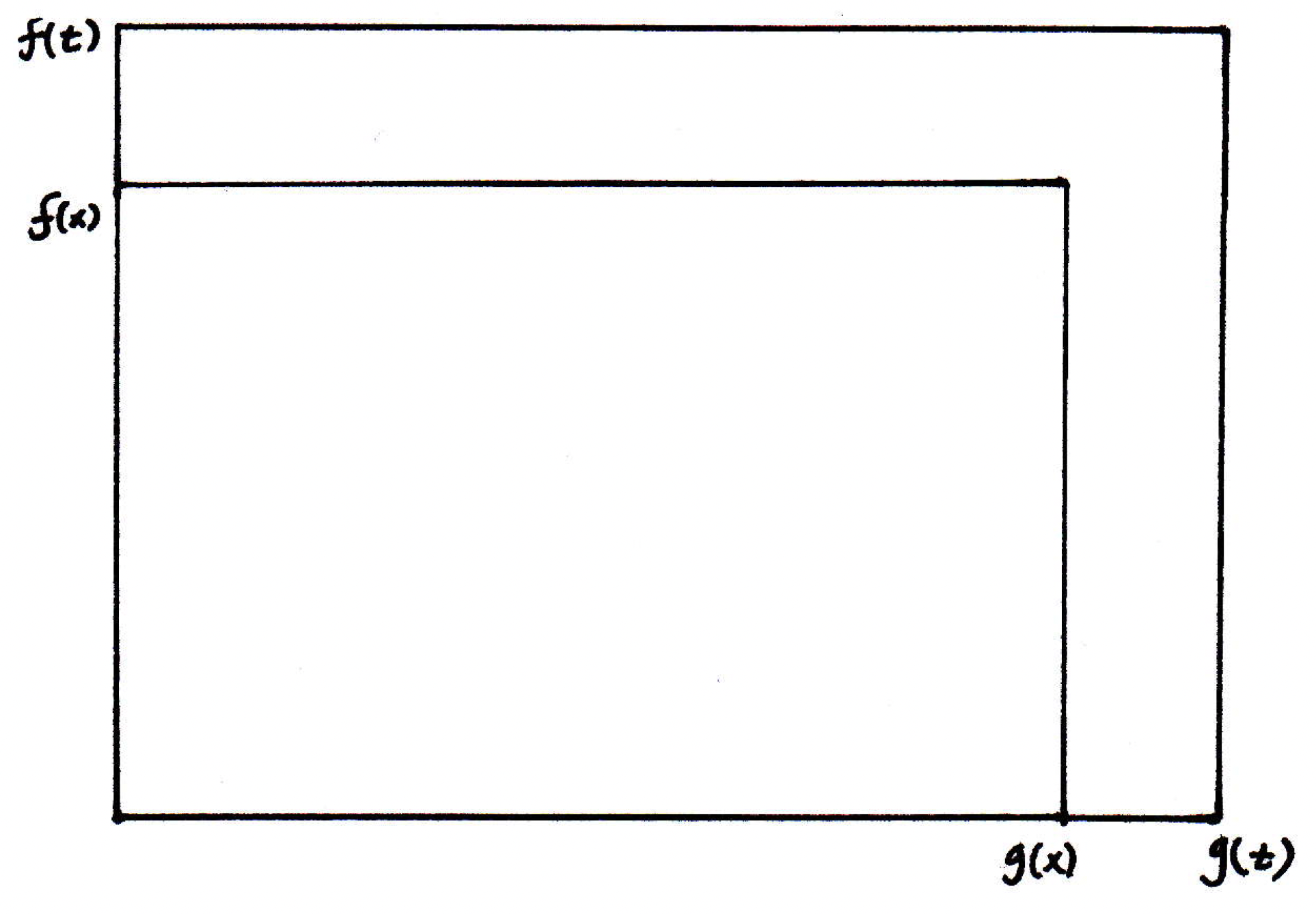
  So the rate of change of $h$ would be looking at the change in the area of the box with respect to the change time. But what is the change in the area of the box? It's just the new region that's been introduced, but this region can be written in terms of two rectangles. So then we have the following:

  $$h(t)-h(x)=\underbrace{g(x)[f(t)-f(x)]}_{\text{rectangle on right}}+\underbrace{f(t)[g(t)-g(x)]}_{\text{rectangle on left}}.$$

  What can we do now? How about divide both sides by $t-x$? We will get the quotient we are interested in and much more; in particular, if we take the limit as $t\to x$, then we get the following:

  $$\lim{t\to x}\frac{h(t)-h(x)}{t-x}=\underbrace{g(x)}_{g}\cdot\underbrace{\frac{f(t)-f(x)}{t-x}}_{f'}+\underbrace{f(x)}_{f}\cdot\underbrace{\frac{g(t)-g(x)}{t-x}}_{g'},$$

  where the $f(t)$ became an $f(x)$ because $f$ is continuous because $f$ is differentiable.

• Pathological functions: We've seen functions that are continuous but not differentiable. If you have a function that is continuous, then must it be differentiable at some point? Not necessarily everywhere. Just at some point. No.

• Pathological functions (theorem): There exist functions $\R\to\R$ that are continuous everywhere but differentiable nowhere. In other words, we have a function that is so jagged that nowhere does it have a derivative. What is an example of one? Consider the following function:

  $$f(x)= \sum_{n=1}^\infty b^n\cos(a^n\pi x),$$

  where $0<b<1$, and $a$ an odd integer, with the provision that $ab>1+\frac{3\pi}{2}$. (The product has to be big enough so that as it gets more jagged and thinner.)

  So what are we adding up? We're adding up a bunch of cosine functions. So they're wavy. Note that $a^n$ impacts the frequency while $b^n$ is the amplitude. As $n$ grows, the curves we are adding up have higher and higher frequencies and smaller and smaller amplitudes. How many of these functions should we add? If we only add finitely many of them, then $f(x)$ is just the sum of continuous functions which is continuous. If $n\to\infty$, as specified above, then $f(x)$ is an infinite sum so pointwise it is a series, but as a collection of functions it is an infinite sum of functions, and you cannot say (as you will see) that infinite sum of a bunch of continuous functions is continuous.

  Our pictures will look something like the following for $n=1,2,3,4,5,6$:

  

  So what we are seeing above are the partial sums of the sum of continuous functions. At each stage, we get a little bit more jaggedness, as illustrated above. Then the claim is that in the limit, because for series we are really looking at a limit of partial sums, namely

  $$f(x)=\lim_{\ell\to\infty}\sum_{n=1}^\ell b^n\cos(a^n\pi x)=\sum_{n=1}^\infty b^n\cos(a^n\pi x),$$

  we see that we'll get something that happens to be verifiably continuous but also verifiably not differentiable.

Mean value theorem

What is the mean value theorem and why is it one of the most important theorems concerning derivatives?

• Motivation: We've talked about what a derivative is, but now we want to know about a theorem that is basically the big workhorse in terms of proving lots of things about derivatives. This theorem is the mean value theorem.

• Mean value theorem (statement): If $f$ is continuous on $[a,b]$ and differentiable on $(a,b)$, then there exists a point $c\in(a,b)$ such that

  $$f(b)-f(a)=(b-a)f'(c). \tag{1}$$

  One way to think about what (1) is the following: Consider a function that looks something like the following:

  

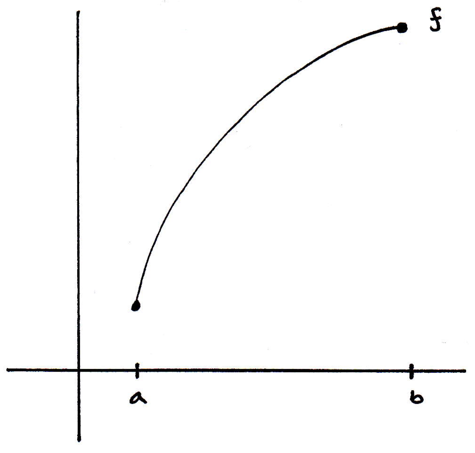
  So if $f$ is continuous on $[a,b]$ and differentiable on $(a,b)$, as illustrated above, then look at what happens when we rewrite $f(b)-f(a)=(b-a)f'(c)$ in the following way (by dividing both sides by $b-a$):

  $$\frac{f(b)-f(a)}{b-a}=f'(c).$$

  What we get then is the slope of the secant line:

  

  And what we're saying is that the slope of this secant line is actually equal to $f'(c)$, where $c\in(a,b)$. Where might such a $c$ be? Well, it looks to be the following:

  

  Here there is only one such $c$, but in general there may be anywhere from just one to infinitely many:

  

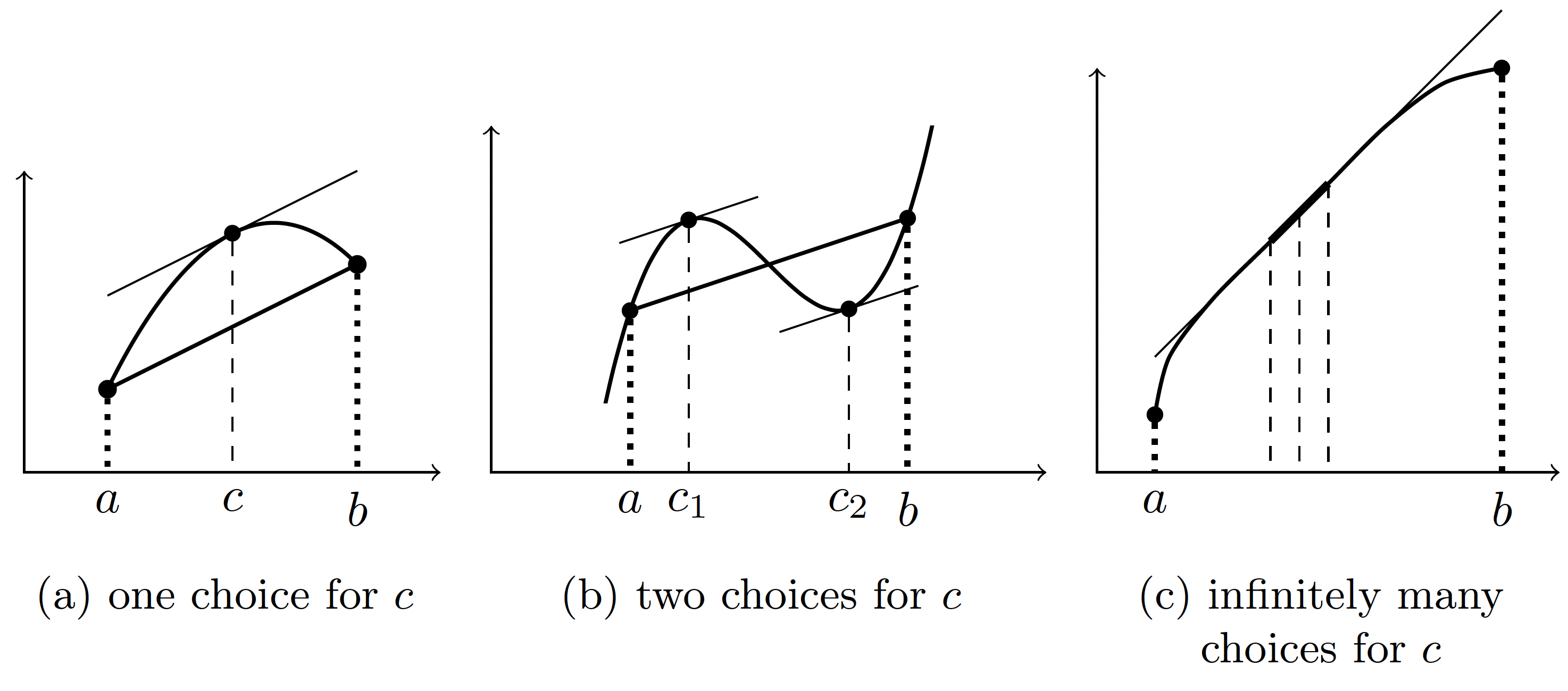
  So basically, the mean value theorem is saying there exists at least one point between the endpoints where the slope of the curve at this point is the same as the slope of the secant line connecting the endpoints of the interval in which $c$ lies.

  Why do we require $f$ be differentiable on $(a,b)$ instead of, say, $[a,b]$? The theorem would certainly be true if we looked at $f$ being differentiable on $[a,b]$ instead of $(a,b)$, but $f$ being differentiable on $(a,b)$ is one of the weakest conditions you can give to ensure that the claim of the theorem holds true. We don't need the derivative limit to exist at the endpoints. We could have a crazy function that doesn't have an endpoint limit (i.e., where the derivative doesn't exist at the endpoint) but the derivative exists everywhere inside.

• Significance of the mean value theorem: What's the big deal about the mean value theorem? Here's the big deal: This is really the only theorem we have that connects the value of the function to the value of the derivative without involving limits. So what (1) does is it connects the value of $f$ to the value of $f'$ (somewhere) without using limits. That's what's nice about this. So anytime you have a statement in calculus that you prove in a sort of hand wavy way, well, if you want to make hand wavy precise, then you go back to the mean value theorem.

• Sample application of mean value theorem: If $f'(x)>0$ for all $x\in(a,b)$, then $f(b)>f(a)$. Let's prove this but not in a hand wavy way.

  What can we say about $f(b)-f(a)$? What are we trying to show about $f(b)-f(a)$? We are trying to show that $f(b)-f(a)>0$. Well, by the mean value theorem, we have

  $$f(b)-f(a)=(b-a)f'(\alpha)$$

  for some $\alpha\in(a,b)$. Do we know which $\alpha$? No. Does it matter though? No. Why? What do we know about $f'(\alpha)$? It must be positive. What about $b-a$? That must also be positive. So we have

  $$f(b)-f(a)=\underbrace{(b-a)}_{>0}\underbrace{f'(\alpha)}_{>0}>0,$$

  as desired.

  You'll see many more applications of this theorem. In fact, pretty much all of the exercises in Chapter 5 of [17] are some version of the mean value theorem. Now let's see why the mean value theorem is true.

• Mean value theorem (proof): How might we gain some intuition as to why this theorem is true? Let's consider a non example first. Suppose we have the following function:

  

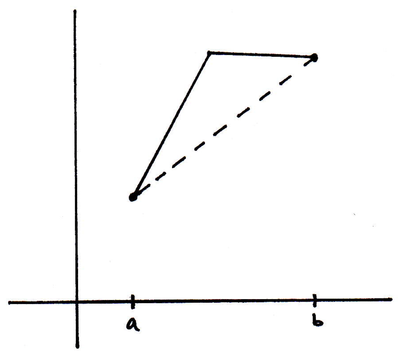
  Is it true that there is a point in between $a$ and $b$ that has the same slope as the pictured secant line? No! What failed? Differentiability on $(a,b)$ failed. Why did it fail? Well, the slopes of the secant lines to the right of the corner are always less than that of $\frac{f(b)-f(a)}{b-a}$; and to the left of the corner, the slopes of the secant lines are always great than $\frac{f(b)-f(a)}{b-a}$. So how can we wrap our heads around the main idea here? Where should we go with our proof? Let's look at a special case first perhaps. We can sort of turn our first non example on its head a bit:

  

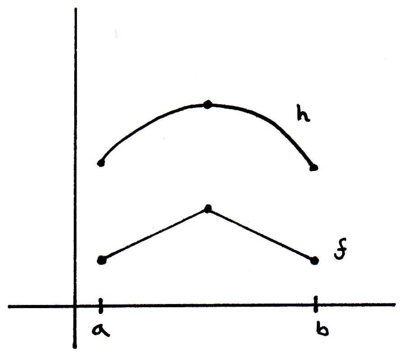
  If $h$ is differentiable, then $h'$ is 0 at its local maximum. Well, why does that fail for $f$ pictured above? At the local maximum of $f$, we see that $f'$ does not exist. So the existence of the derivative will help somehow. What can we say about a local maximum? Here's the idea: If $h$ on $[a,b]$ has a local max at $c\in[a,b]$ and $h'(c)$ exists, then $h'(c)=0$. This is actually not hard to show. Here's the idea: Just take a look at what you are taking the limit of:

  $$\frac{h(t)-h(c)}{t-c}.$$

  If $h$ has a local maximum at $c$, then what must be true of $h(t)-h(c)$ regardless of which side you are on? It must be the case that $h(t)-h(c)<0$ because $c$ is the location of a local maximum. What about $t-c$? Here it depends on what side you are on. What we see is that

  $$\frac{h(t)-h(c)}{t-c}$$

  will be negative on the right (i.e., if $t>c$) and positive on the left (i.e., if $t<c$). So when we look at

  $$\lim_{t\to c}\frac{h(t)-h(c)}{t-c},$$

  we are taking the limit where we get a bunch of positive numbers on the left and a bunch of negative numbers on the right. If that limit exists, then what has to be true? The left- and right-hand limits have to exist and be equal. So if you take the limit of a bunch of positive numbers, then the only values the limit could be are 0 or larger than that. Similarly, if you take the limit of a bunch of negative numbers, then the only values that the limit could be are 0 or smaller than that. So what's the only thing this derivative could be if it exists? It would have to be 0. That's the argument. That is, given that $h$ has a local max on $[a,b]$ at $c\in[a,b]$ and $h'(c)$ exists, then

  $$\lim_{t\to x^+}\frac{h(t)-h(c)}{t-c}<0 \qquad\text{and}\qquad \lim_{t\to x^-}\frac{h(t)-h(c)}{t-c}>0.$$

  Since $h'(c)$ exists, the limits above must exist and be equal to each other. Hence, $h'(c)=0$, as desired. This is a simple version that is called Rolle's Theorem.

• Mean value theorem (proof): Suppose Rolle's Theorem is true. How will this enable us to prove the mean value theorem? Well, how is the picture

  

  like

  

  in some ways? It's just a little off. If we wanted to apply the mini result (i.e., Rolle's theorem) to a general picture, then we should just take the function and subtract off the secant line. Then you get a new function $h$ that has the requisite properties. This is just in words, but the proof can be carried out with relative ease. Let's prove an even more general result.

• Generalized mean value theorem: If $f(x)$, $g(x)$ are continuous on $[a,b]$ and differentiable on $(a,b)$, then there exists $c\in(a,b)$ such that

  $$[f(b)]-f(a)]g'(c)=[g(b)-g(a)]f'(c). \tag{2}$$

  It should be noted that we know nothing about the location of the $c$ above.

  Why is the above result called the generalized mean value theorem? Note that if $g(x)=x$, then we simply get the mean value theorem because $g'(x)=1$ in that case. So we'll prove the general mean value theorem using Rolle's Theorem, and this will handle the mean value theorem.

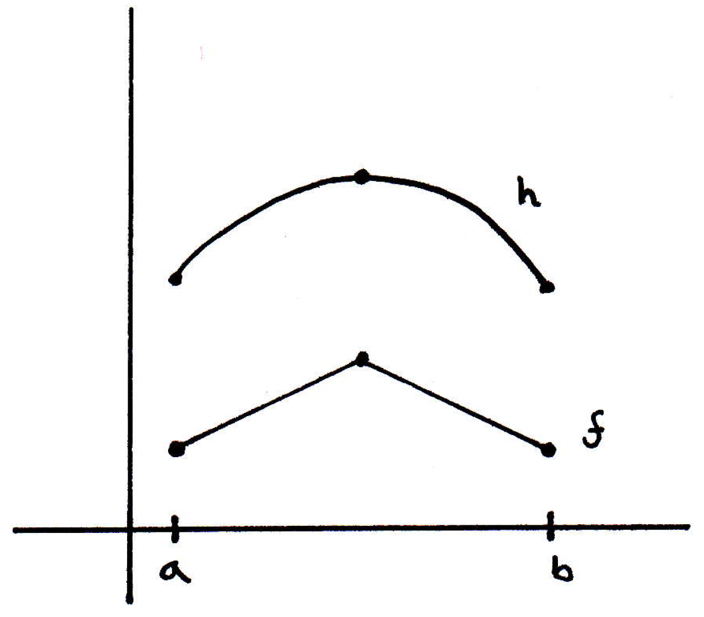
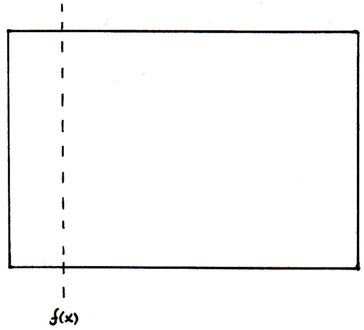
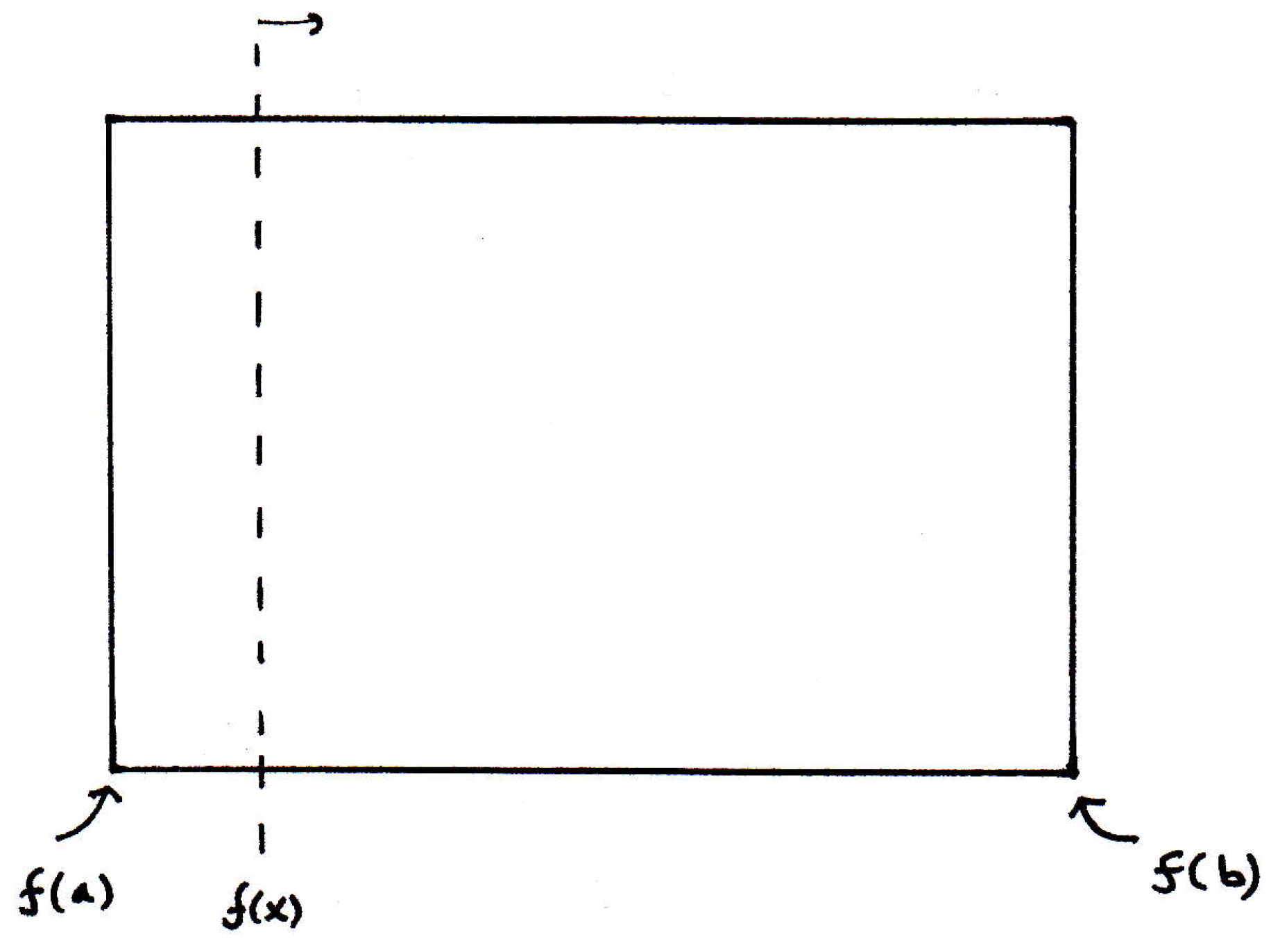
• Generalized mean value theorem (proof): Suppose we have a cake that looks like so:

  

  And suppose we have a knife that is going to sweep over the cake from left to right, and the position of the knife is given by a function $f$:

  

  The knife may not even go left to right, but the point is that the position of the knife is given by $f$ even though you can imagine sweeping it from one side to the other so that at time $a$ it is at $f(a)$ and at time $b$ it is at $f(b)$:

  

  Suppose, simultaneously, we have another knife whose position is given by $g(t)$:

  

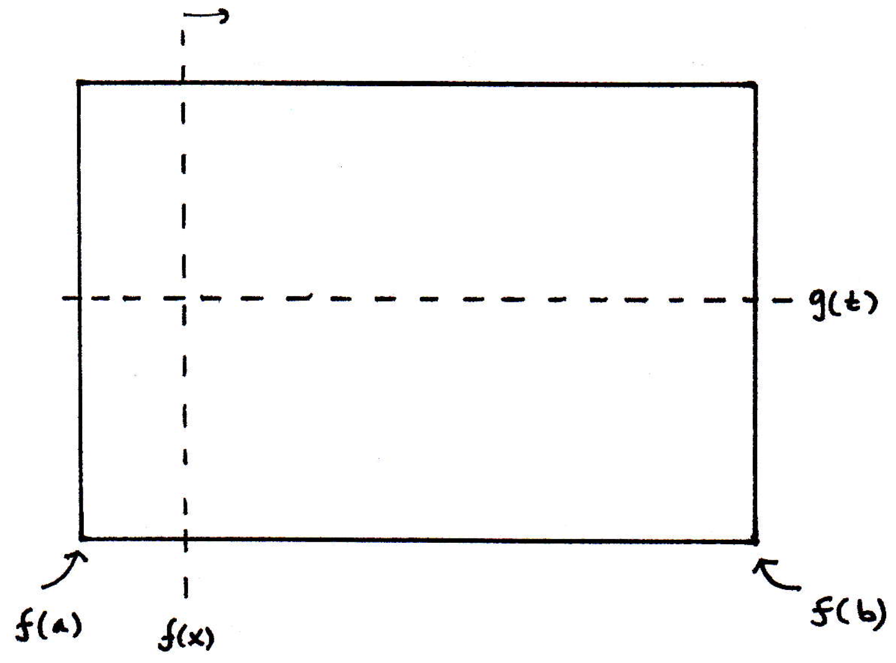
  Also, at time $a$ it's at the bottom, and at time $b$ it's at the top:

  

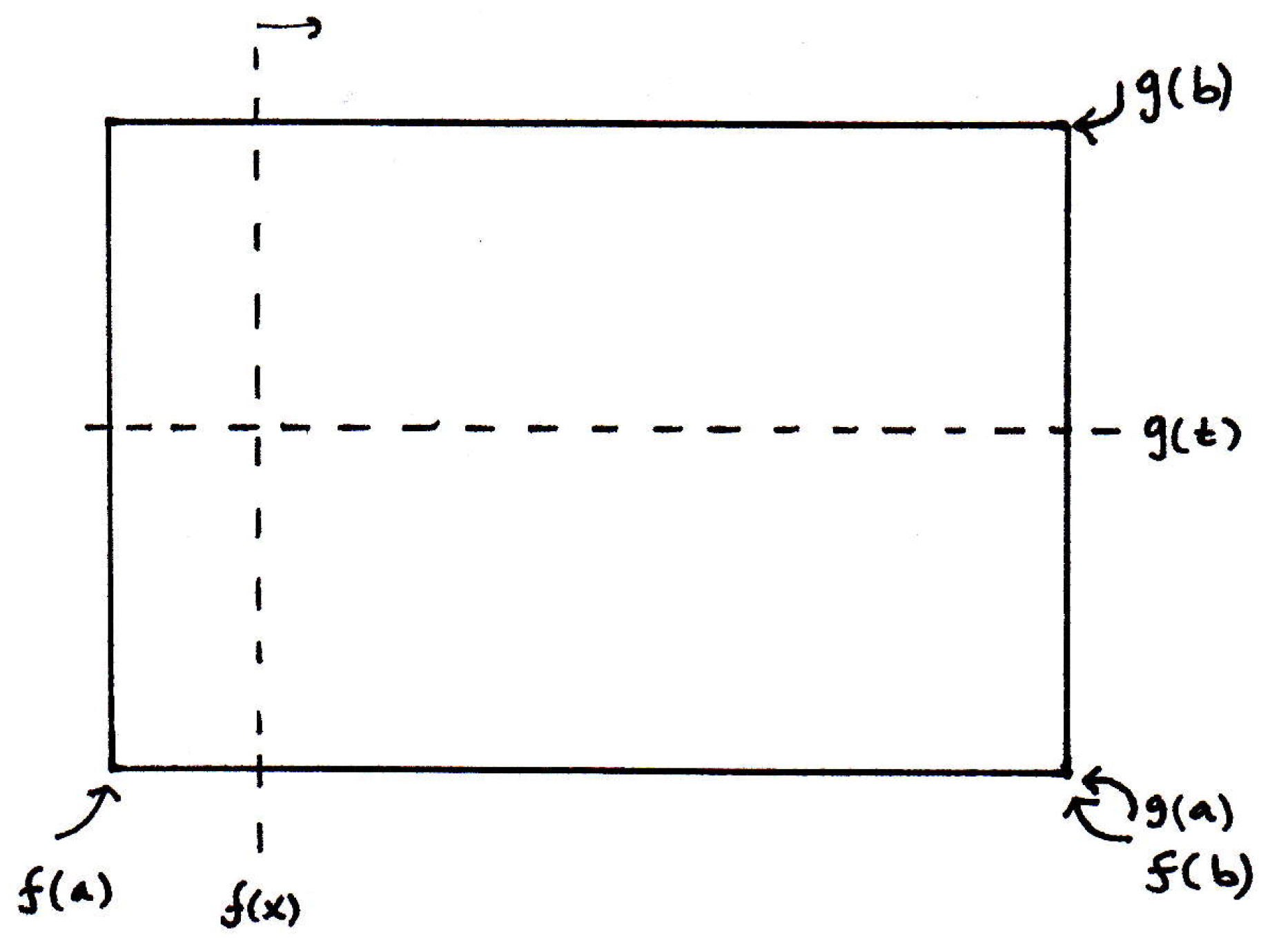
  Let's call the $f$ knife $K$ and the $g$ knife $L$ for ease of reference:

  

  We claim that the left-hand side of (2) is the rate that knife $L$ sweeps out area of cake. (We see that $f(b)-f(a)$ is the distance multiplied by the rate at which the knife $L$ is sweeping out length. So the product $[f(b)-f(a)]g'(c)$ is the rate at which knife $L$ sweeps out area of cake.) Similarly, the right-hand side of (2) is the rate at which $K$ sweeps out area. (We have $g(b)-g(a)$ which is the width times the rate of change that the knife $K$ is sweeping out width. So the product $[g(b)-g(a)]f'(c)$ is the rate at which knife $K$ sweeps out area.) So what, then, is the generalized mean value theorem saying in terms of knives and areas??

  Imagine knife $K$ starts at one end and moves to the other end, and knife $L$ simultaneously starts at one end and moves to the other end. When they both start, they've swept out no area. When they've both ended, they've swept out the complete cake. What this theorem is saying is that if they both sweep out the total area in the same interval $[a,b]$, then at some point their rates must be the same. Why? Because if one knife were sweeping out more area than the other, at a greater rate, then it couldn't be the case that they both start and end and sweep out the same area. That's basically what it's saying.

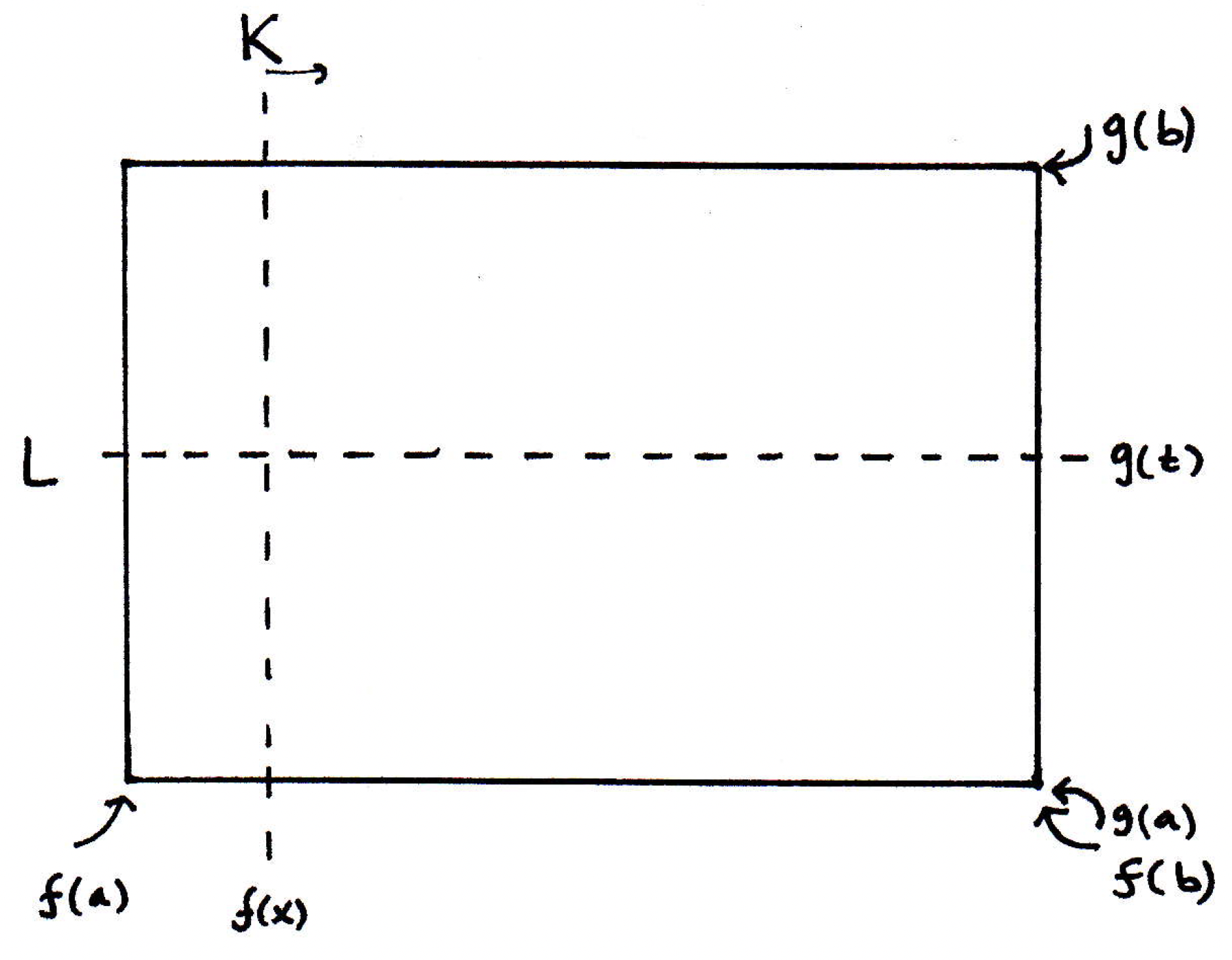
  If you see the above, then you see exactly which function to apply $h$ to. Consider $h(x)=[f(b)-f(a)]g(x)-[g(b)-g(a)]f(x)$, where $h$ is the difference in the areas swept by time $x$ in our cake picture. That's the function to look at. Why? It's clear that at time $a$, when both knives start, that $h(a)=0$. It's also clear that by the time they both finish the difference in area swept out is also 0; that is, $h(b)=0$. So if you have a function $h$ that starts at 0 and ends at 0, then what can you conclude about that function? We have no idea what this function looks like but that it starts at 0 and ends at 0:

  

  It could look something like the following:

  

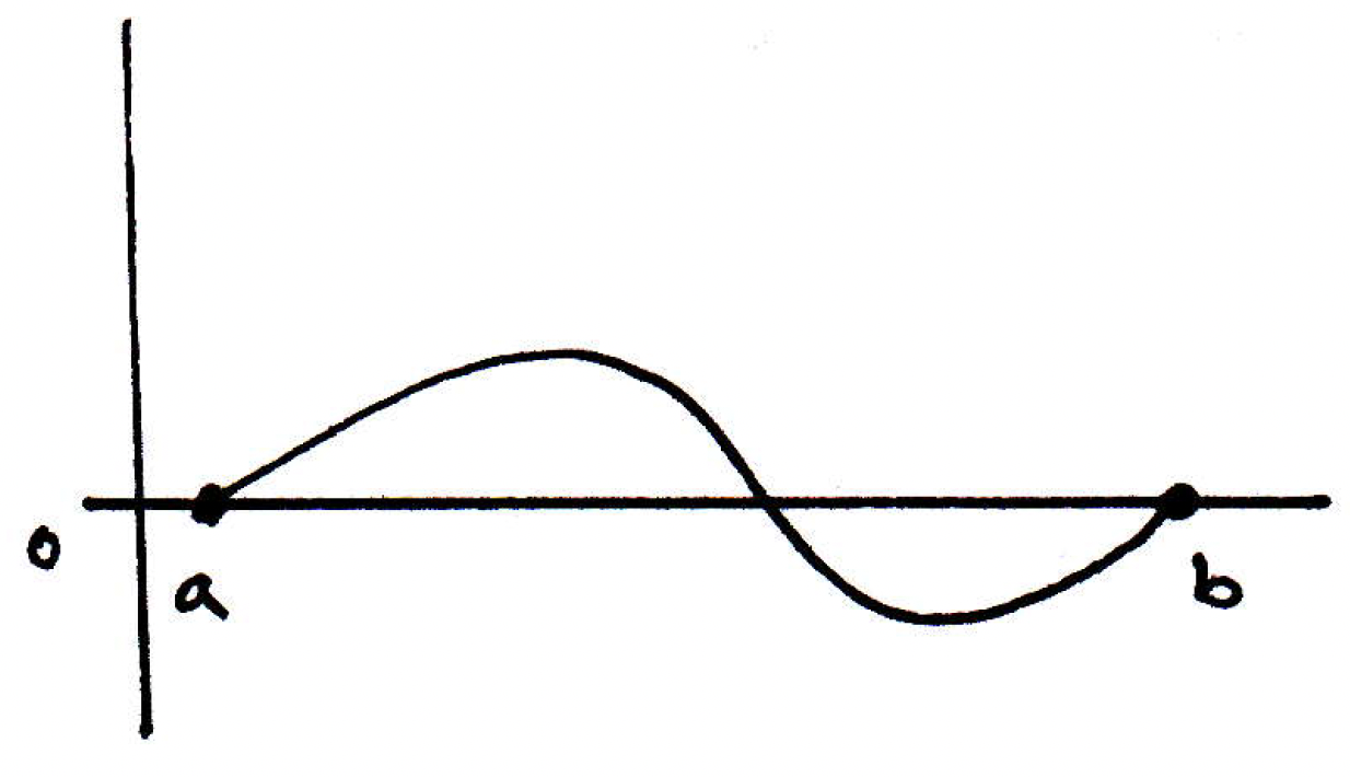
  Regardless, it must have either a maximum or minimum, but by Rolle's Theorem there is some point $c$ where $h'(c)=0$. But $h'(x)=[f(b)]-f(a)]g'(c)-[g(b)-g(a)]f'(c)$. That's the argument. The book basically just gives you the end result (i.e., the expression directly above for $h'(x)$), but here you have the intuition now as to where this argument is coming from.

• Preview of next time: The generalized mean value theorem is basically the workhorse to do almost all of the problems in Chapter 5 in [17]. Next time we will deal with one other theorem that has to do with derivatives, and that theorem is Taylor's Theorem, and it wouldn't surprise you that Taylor's Theorem is proved using the mean value theorem.