21 - Continuous functions

Repetition

These lecture notes are slightly repetitive with those of the previous lesson except here we do prove Theorem 4.8 in Rudin. It just takes a while longer to get there.

Where we left off last time

• Recap: Last time we said what it means for a function to be continuous. To say the function $f\colon X\to Y$ is continuous means the following:

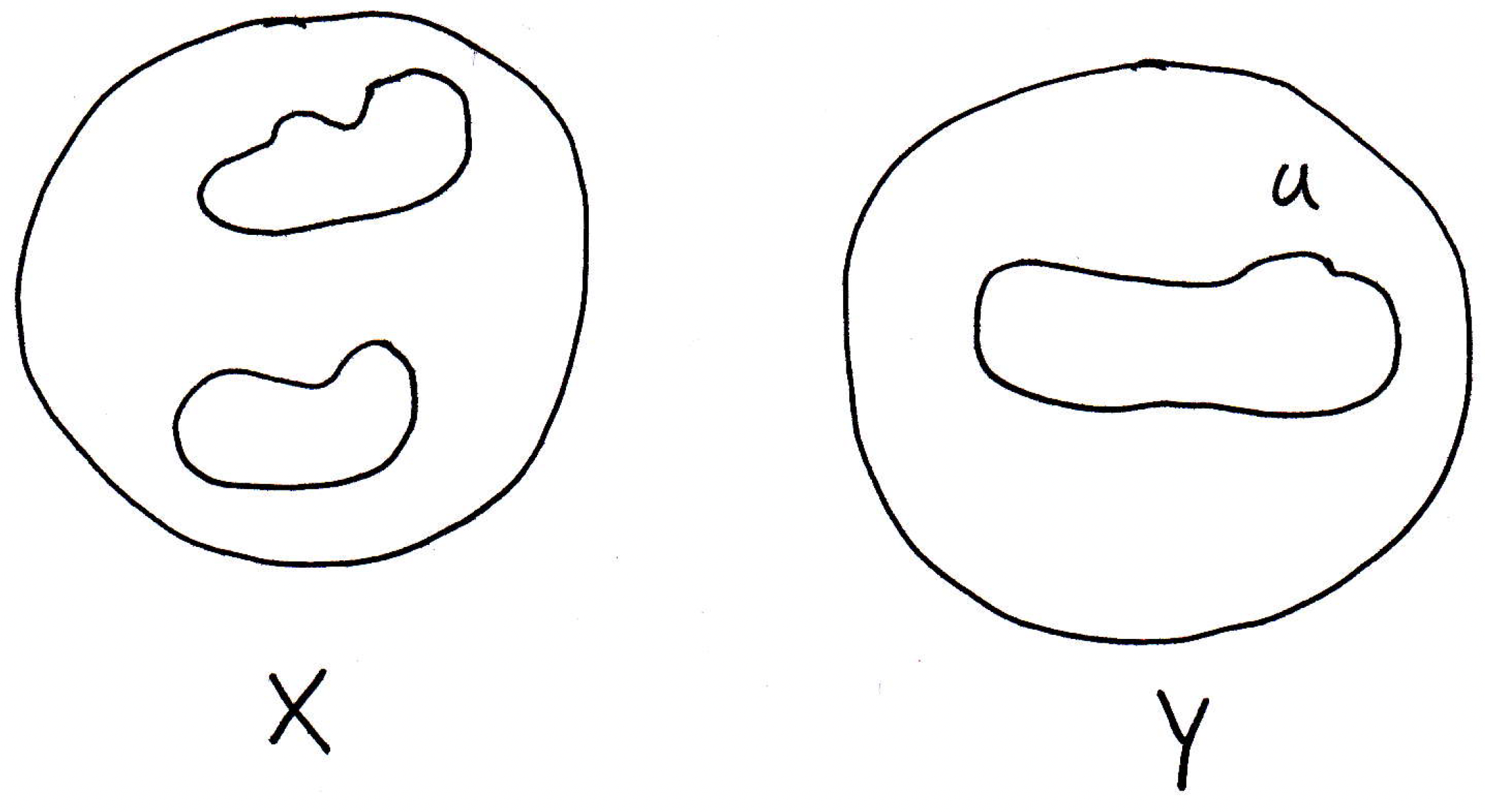
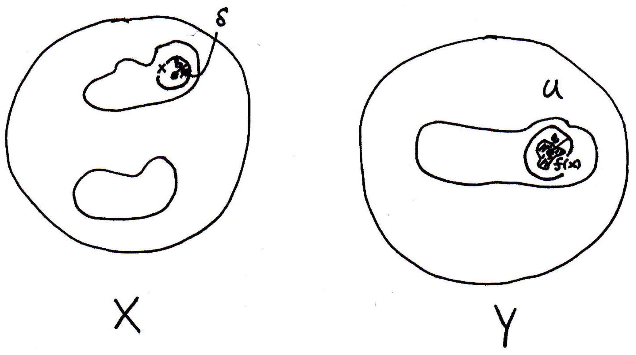
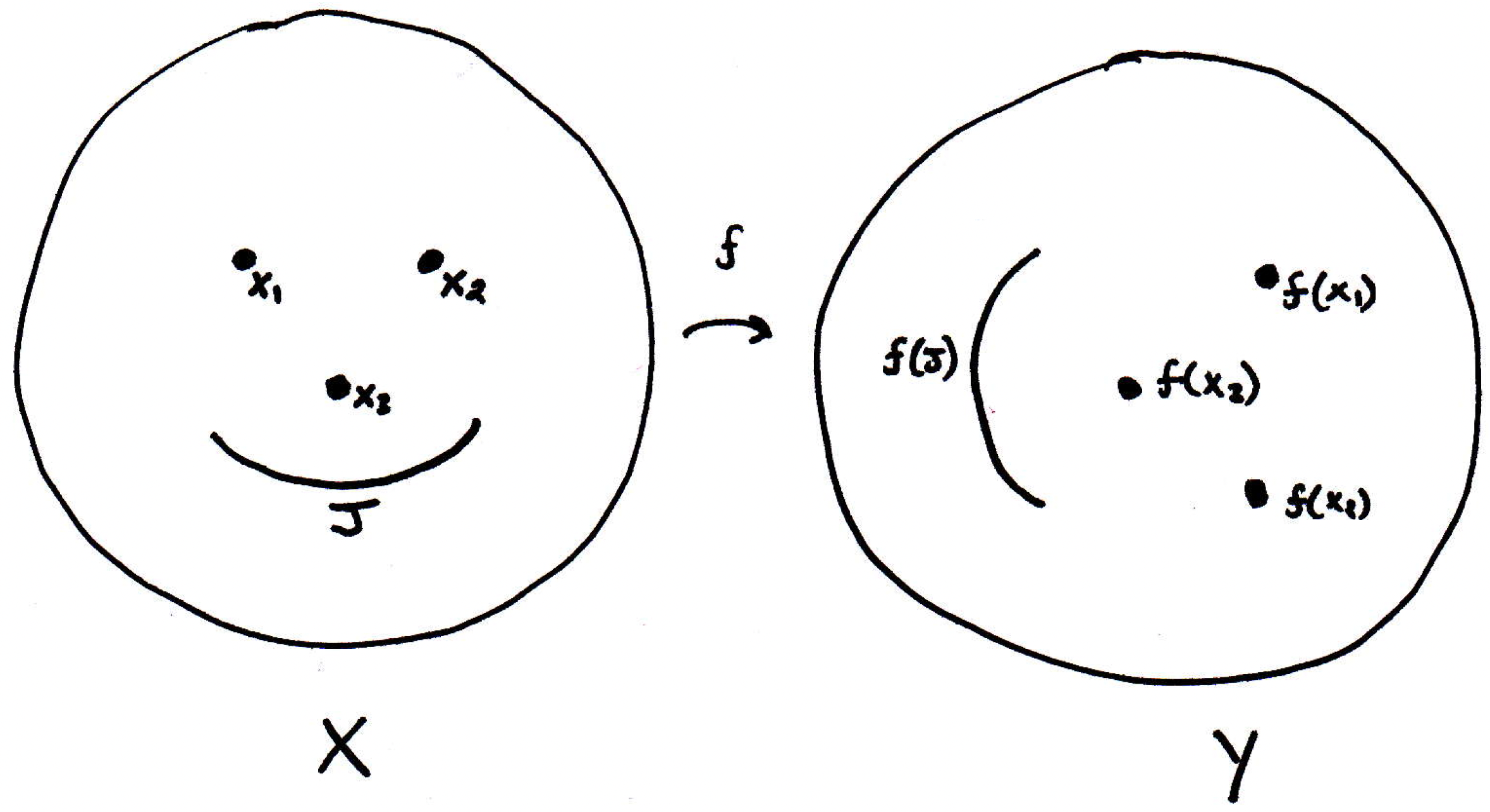
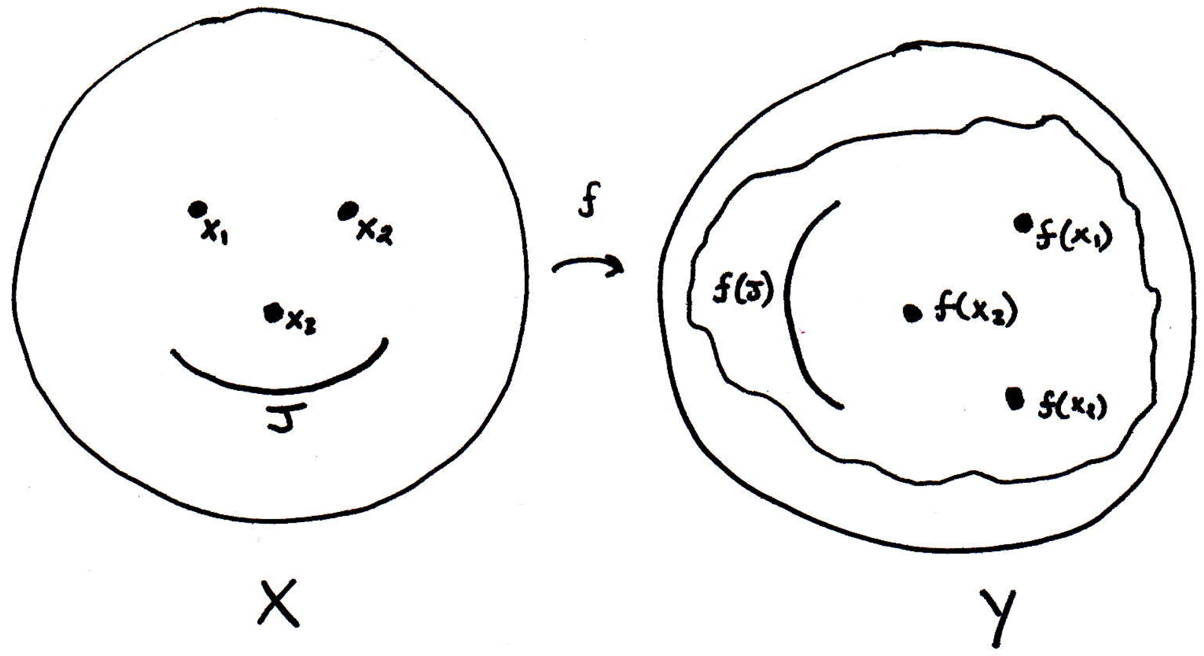
  • Closeness: At each $p\in X$, for every $\epsilon>0$, there is a $\delta>0$ such that there exists $x\in X$ where $d_X(x,p)<\delta$ implies that $d_Y(f(x),f(p))<\epsilon$. That is, close enough points map to close points. That is, you have some function that is taking some space $X$ into some space $Y$, and we want to say it's continuous if it doesn't tear the space up in some way. For example, you could have a function that looks something like the following (poorly drawn but idea is face is split in half and separated):

    

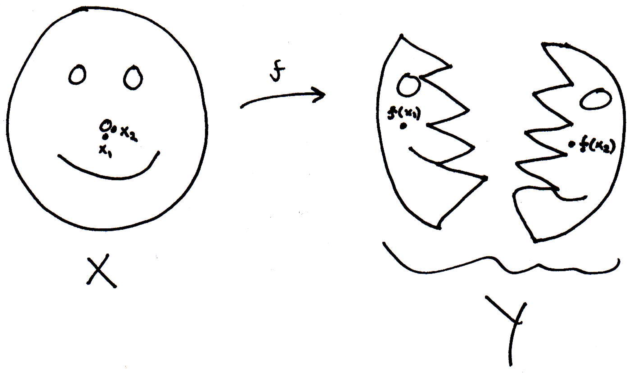
    The above would not be a continuous function. Why is that? Well, because, morally speaking, there are close points in $X$, as $x_1$ and $x_2$ pictured above, which get mapped far away in some sense, namely to $f(x_1)$ and $f(x_2)$.

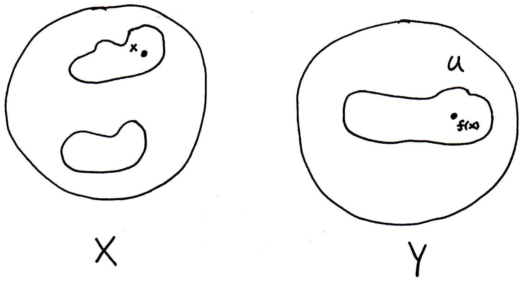
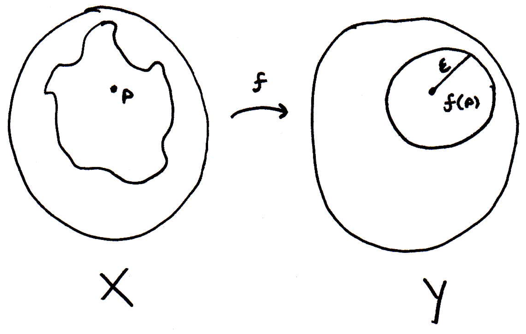
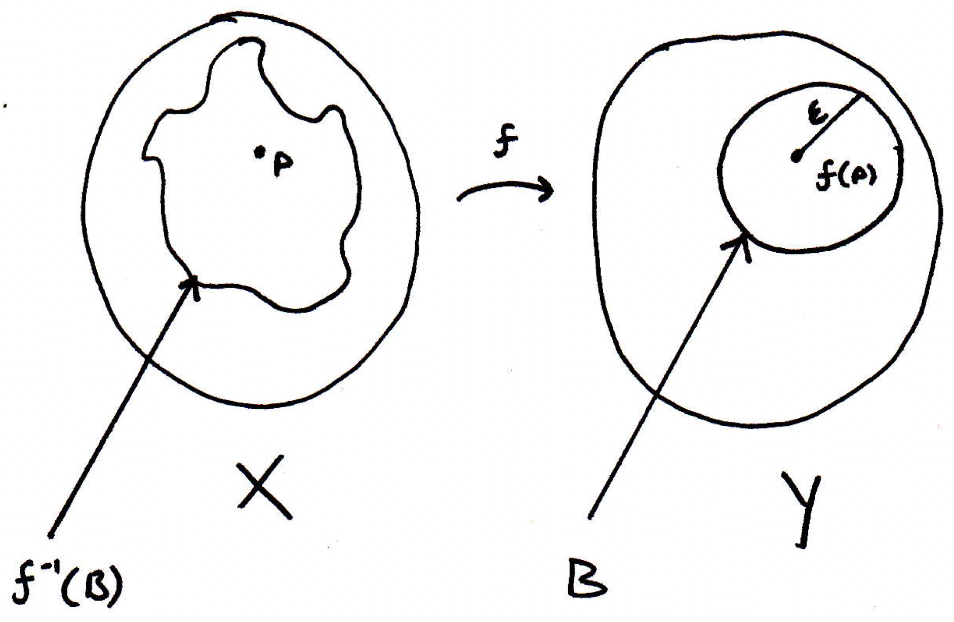
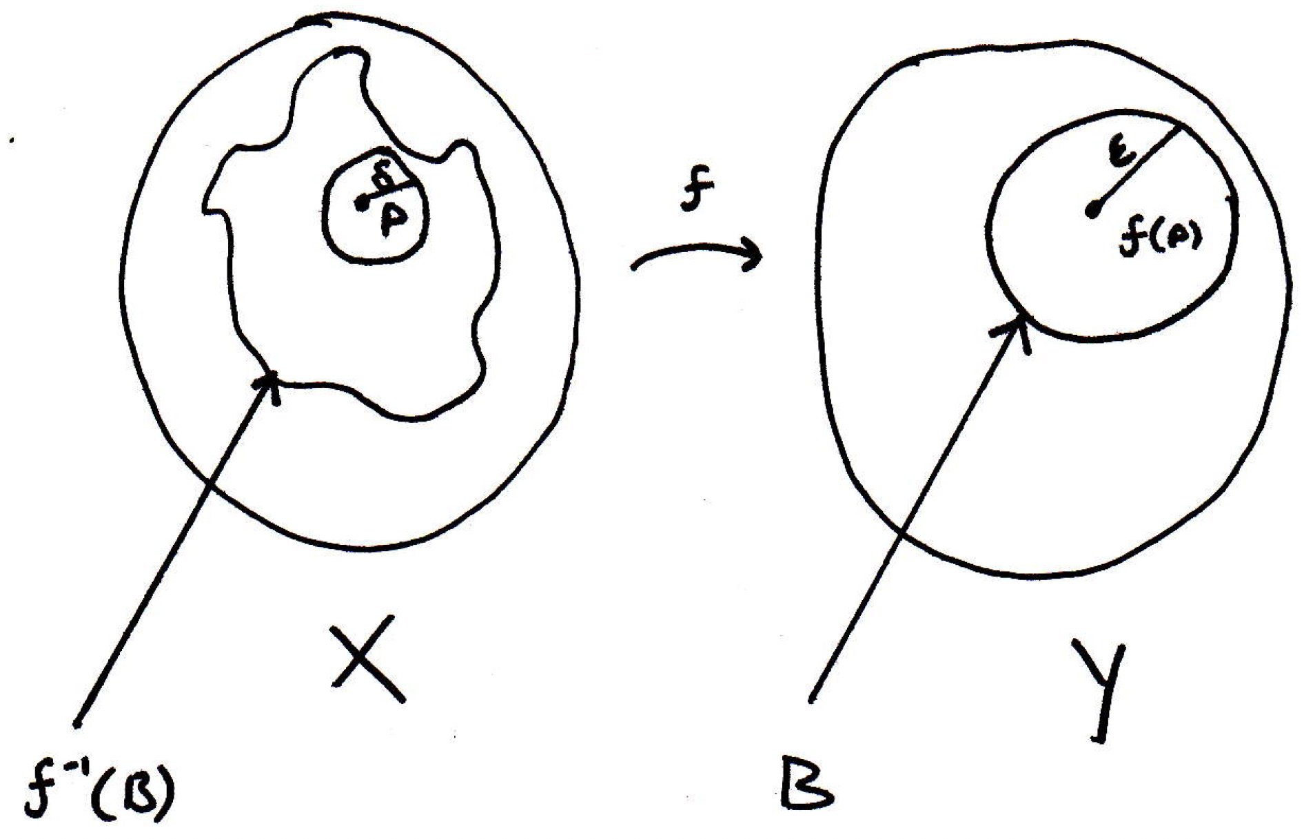
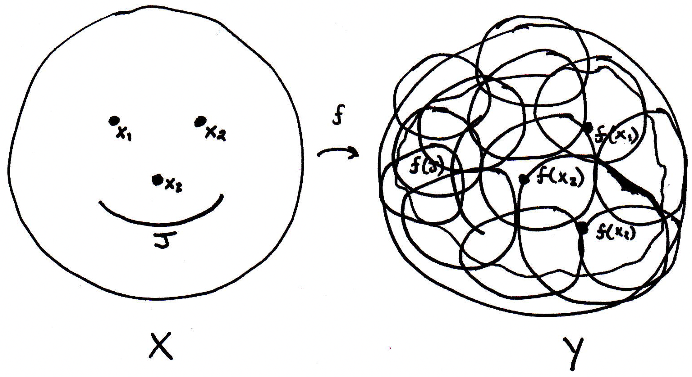
    To be a little more precise, we want to say this function is continuous at a point $p$ if no matter how close you are in the codomain you can find a ball in the domain such that if you're within a ball from point $p$ then the image is within that $\epsilon$ of the image of $p$. So let's try to model this with our picture:

    

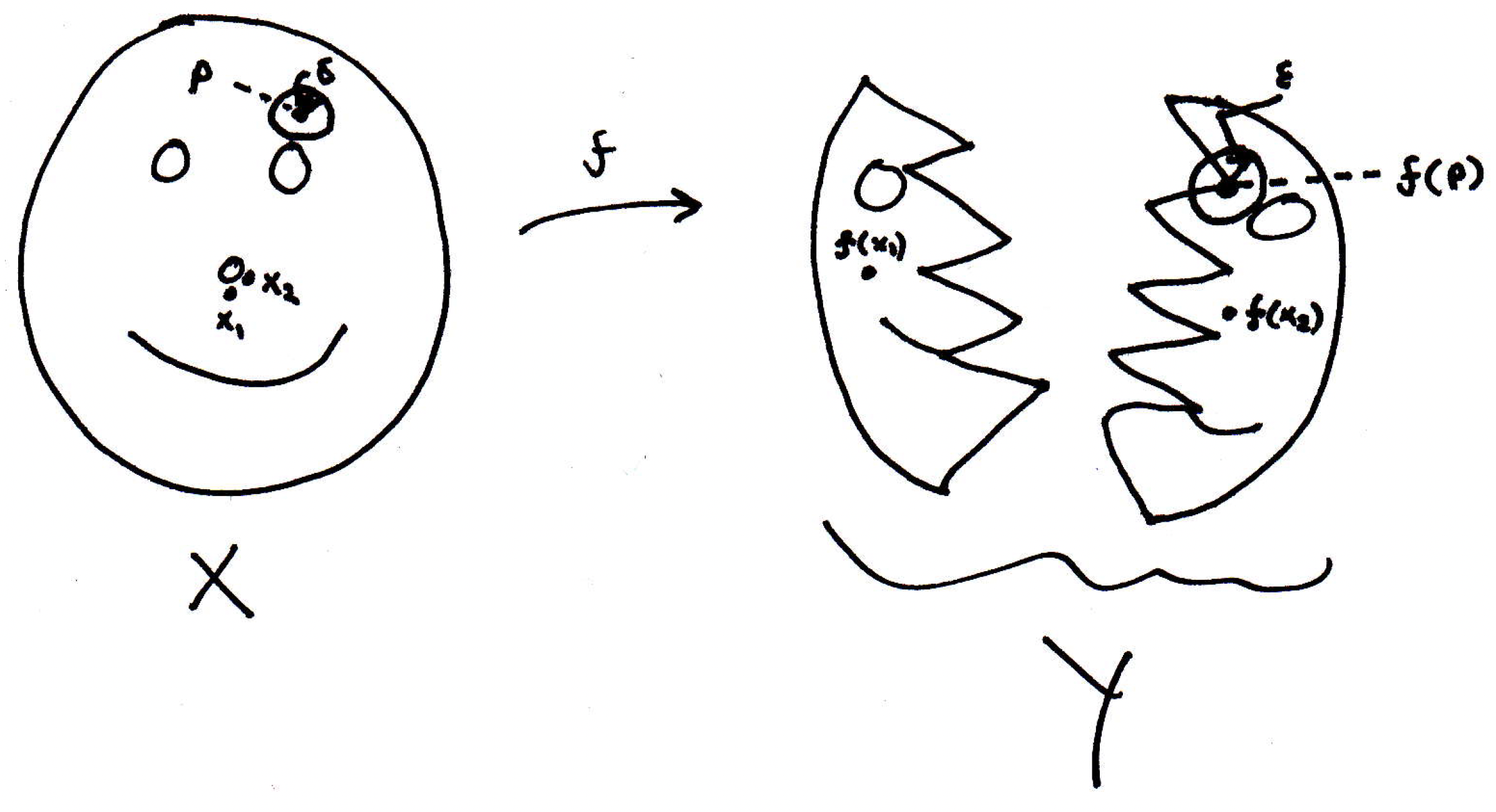
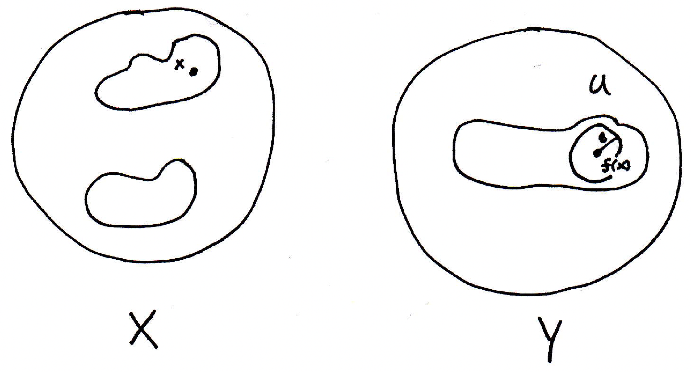
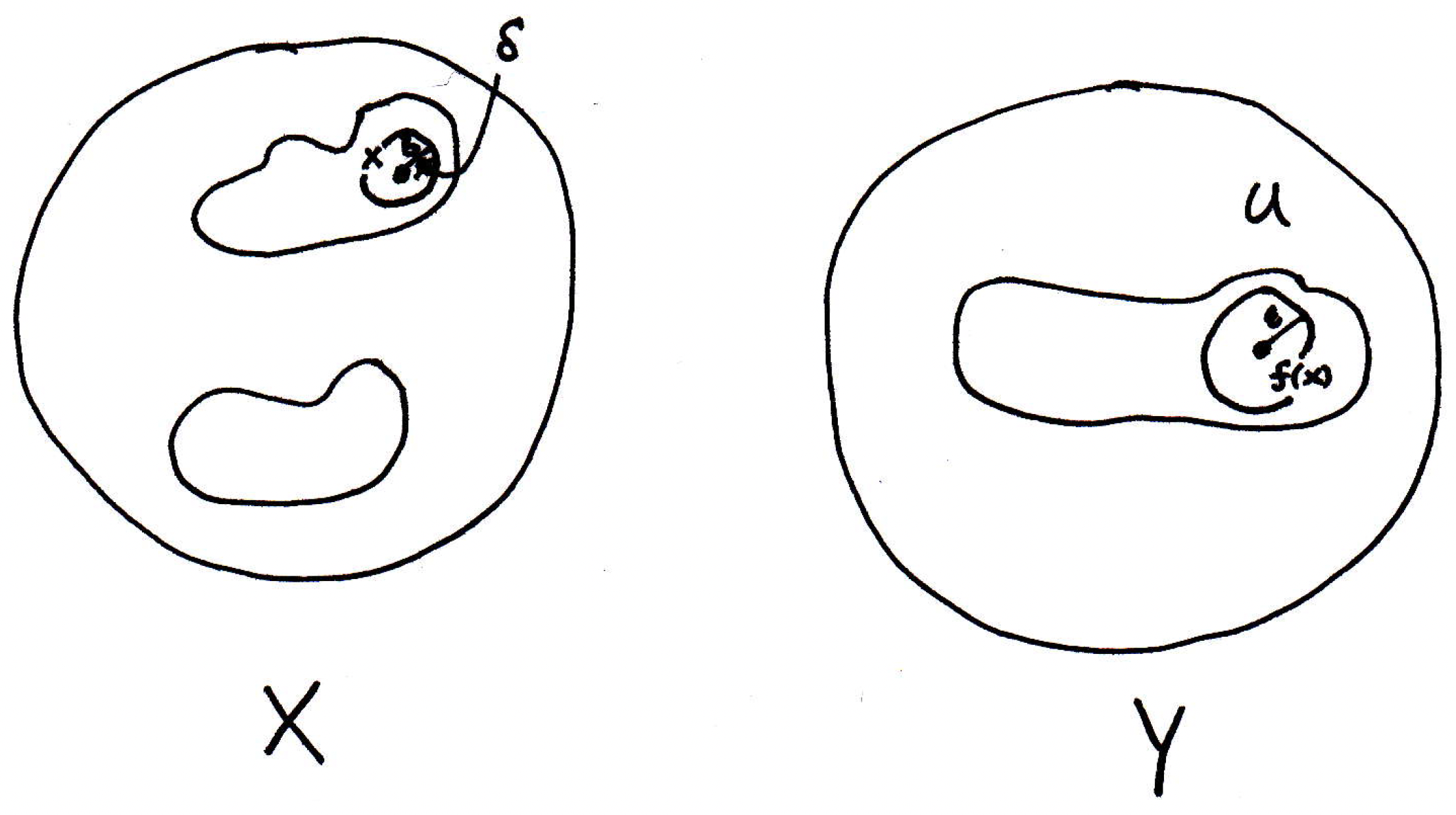
    Is $f$ continuous at $p$ for the $p$ chosen above (the drawing is bad but the idea should still come across)? No. Why not? Well, not the entire image of everything in the $\delta$-ball ends up in the $\epsilon$-ball (the slight corner that's missing):

    

    So we'd say no, the function $f$ is not continuous at the pictured $p$ because there is an $\epsilon$-ball (such as the one pictured) such that there is no $\delta$-ball around $p$ that will map entirely into the $\epsilon$-ball.

  • Sequences: Just to make this connection more integrated with some of the things we have seen, we also saw there was a sequence version of continuity as well, namely the following: For every convergent sequence $\{x_n\}$ in $X$, we have

    $$\lim_{n\to\infty}f(x_n)=f\Bigl(\lim_{n\to\infty} x_n\Bigr);$$

    that is, the limit of the images is the image of the limit. (Continuous functions preserve limits.)

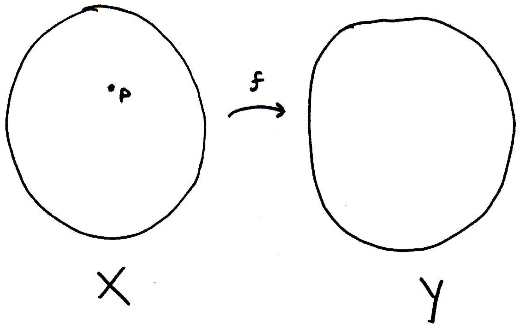
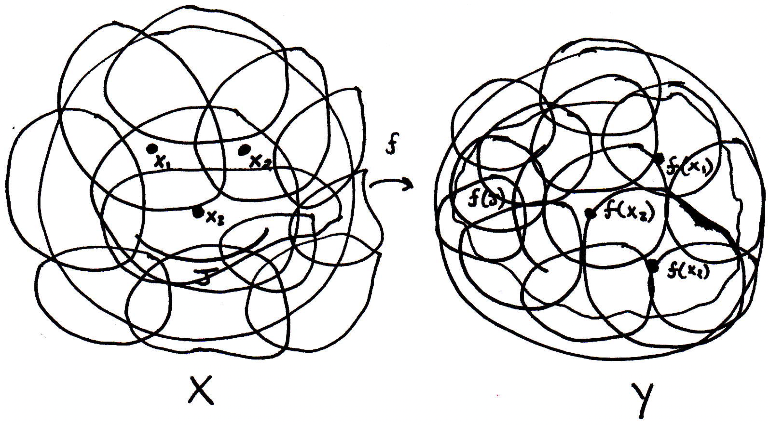
    In our picture, let's pick a point where we think the function $f$ is continuous. How about the point $t$:

    

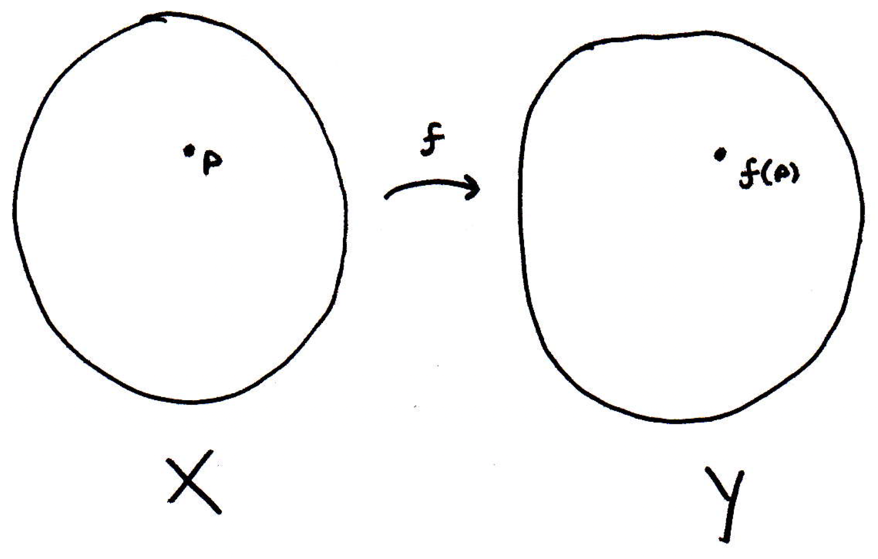
    So if we look at sequences that actually converge to $t$, let's call those points $t_n$, then is it the case that their images, $f(t_n)$, converge to $f(t)$? If the answer is yes for all such sequences, then the function is continuous at that point $t$.

Topological definition of continuity

What was the topological definition of continuity and how do we prove it?

• Theorem statement: The function $f\colon X\to Y$ is continuous if and only if for every open set $U$ in $Y$ we have that $f^{-1}(U)$ is open in $X$.

• Remark about inverse images or preimages: Worth noting is to recall how the inverse image (also called the preimage) is defined: $f^{-1}(U)=\{x \mid f(x)\in U\}$. So the inverse image is the set of all points that get mapped into $U$. Particularly worth noting is that the inverse image need not be a function (the inverse $f^{-1}$ is a function if and only if $f$ is one-to-one and onto). More precisely, if $f\colon X\to Y$ is any function (not necessarily invertible), then the inverse image or preimage of an element $y\in Y$ is the set of all elements of $X$ that map to $y$:

  $$f^{-1}(\{y\})=\{x\in X : f(x)=y\}.$$

  The preimage of $y$ can be though of as the image of $y$ under the (multivalued) full inverse of the function $f$. Similarly, if $S$ is any subset of $Y$ (just like we are dealing with an open set $U$ as a subset of $Y$ in our theorem), then the inverse image of $S$ is the set of all elements of $X$ that map to $S$:

  $$f^{-1}(S)=\{x\in X : f(x)\in S\}.$$

  For example, take a function $f\colon\R\to\R$ defined by $f(x)=x^2$. This function is not invertible. Yet inverse images may be defined for subsets of the codomain:

  $$f^{-1}(\{1,4,9,16\})=\{-4,-3,-2,-1,1,2,3,4\}.$$

  The inverse image of a single element $y\in Y$, namely the singleton set $\{y\}$, is sometimes called the fiber of $y$. When $Y$ is the set of real numbers, it is common to refer to $f^{-1}(\{y\})$ as a level set.

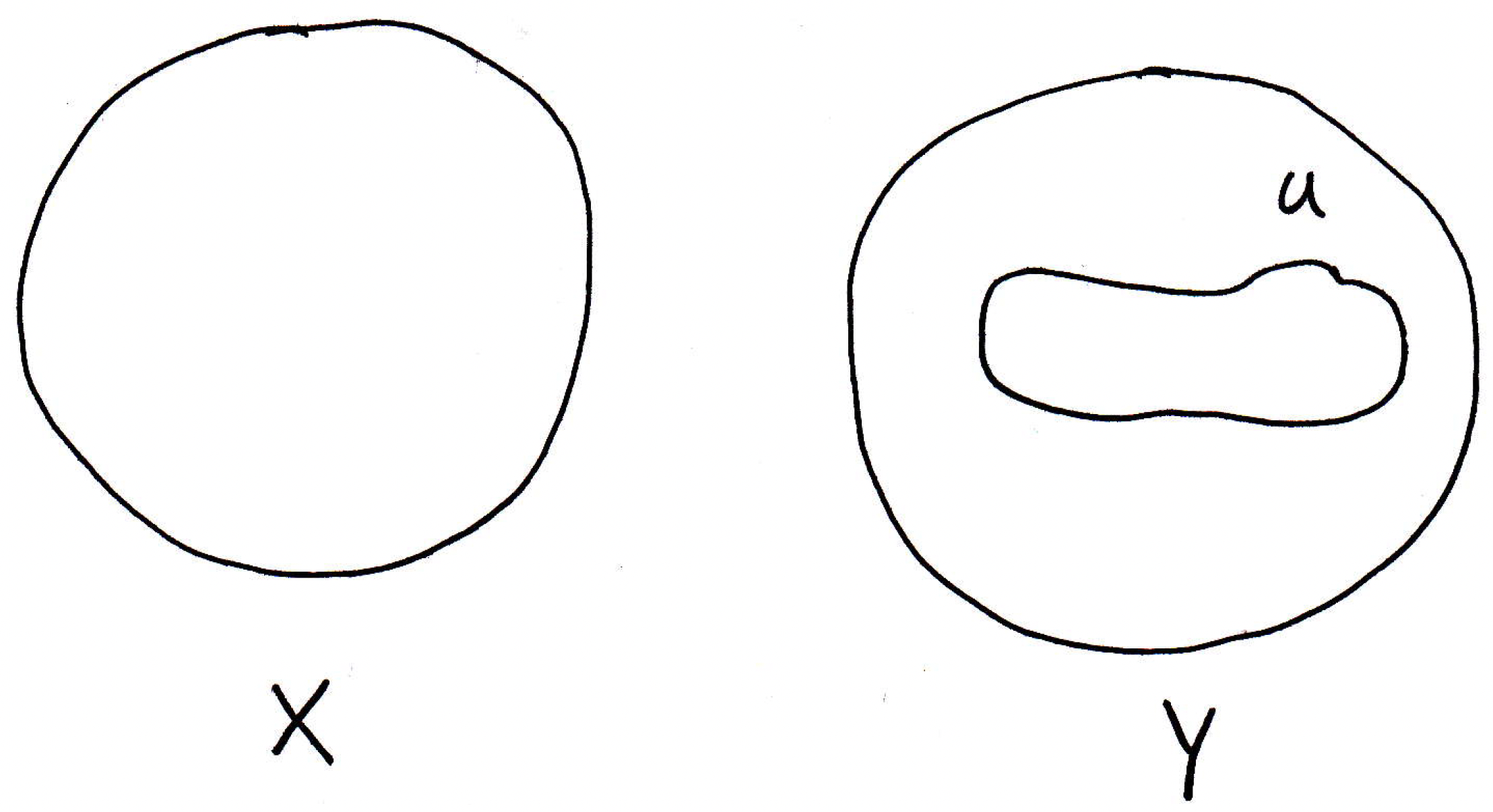
  In our context, maybe we have the following picture:

  

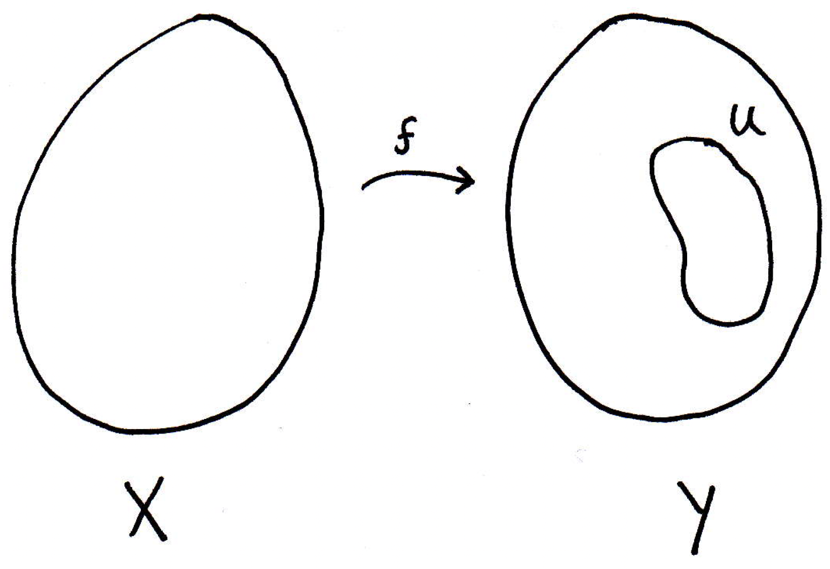
  We could ask what the inverse image of $U$ is here. What is that? It will be the set of all points in $X$ that are mapped into $U$. As noted above, the function $f$ may not actually have a corresponding inverse function, but the image of $f$ will have an inverse image. Consider the following picture:

  

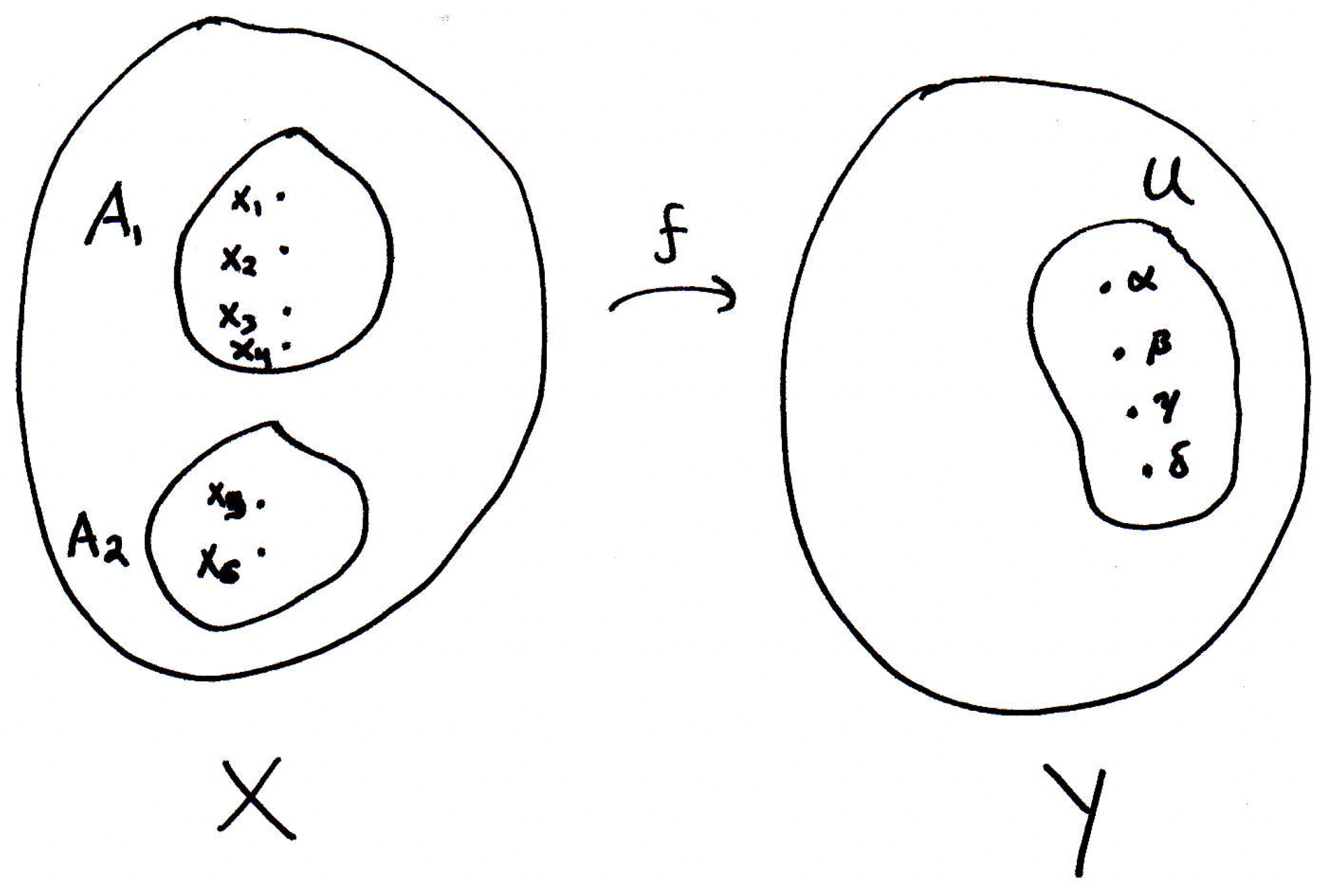
  Suppose we have the following mappings:

  $$\begin{align*} x_1 &\stackrel{f}{\mapsto} \alpha\\[0.5em] x_2 &\stackrel{f}{\mapsto} \beta\\[0.5em] x_3 &\stackrel{f}{\mapsto} \gamma\\[0.5em] x_4 &\stackrel{f}{\mapsto} \delta\\[0.5em] x_5 &\stackrel{f}{\mapsto} \delta\\[0.5em] x_6 &\stackrel{f}{\mapsto} \delta \end{align*}$$

  We see that the inverse image of $U$ is $f^{-1}(U)=\{x_1,x_2,x_3,x_4,x_5,x_6\}$ even though $x_4$, $x_5$, $x_6$ all map to $\delta$. So the function $f\colon A_1\cup A_2\to U$ would not have an inverse function. However, the function $f\colon A_1\to U$ would have an inverse function.

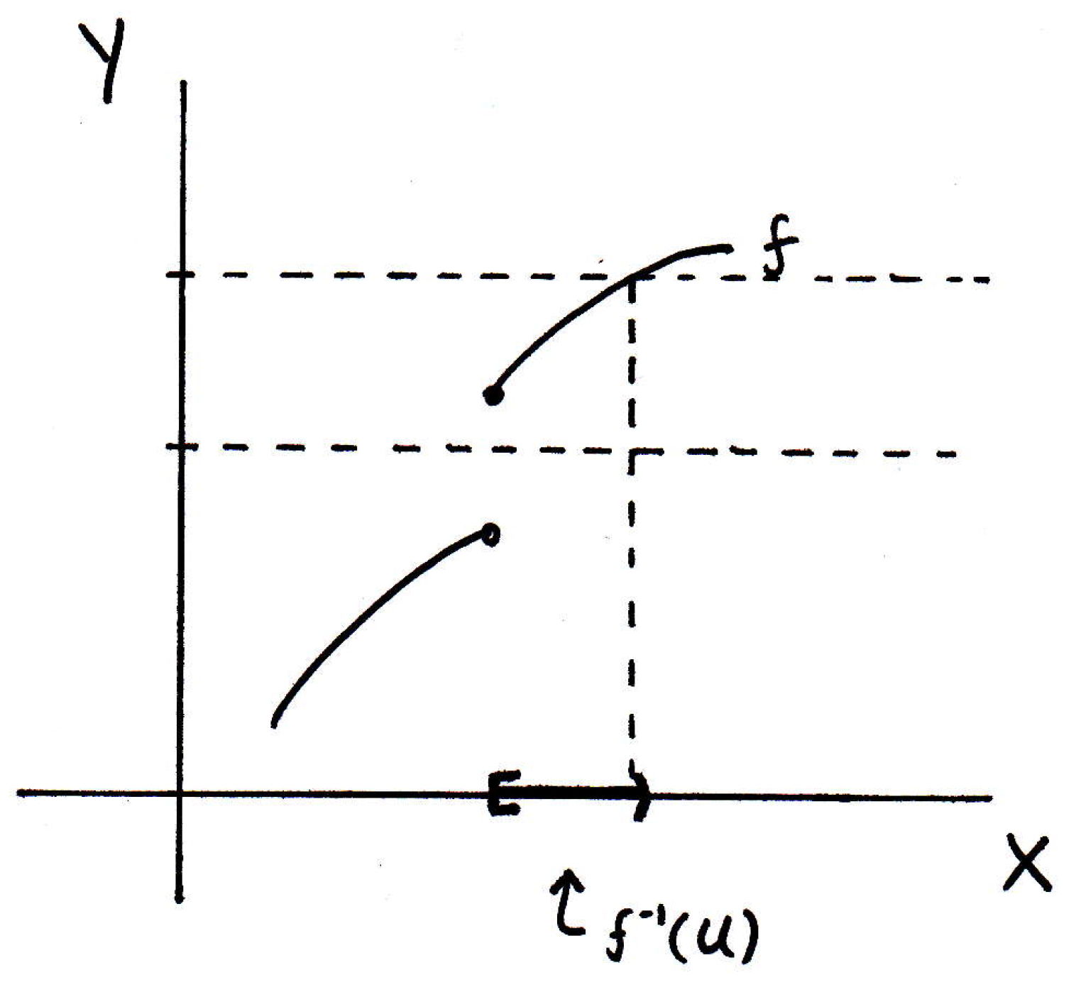
• Revisiting theorem: What does it mean for a function to be continuous? We claim it's equivalent to saying the inverse image of any open set $U$ in $Y$ is open. Let's consider the following picture of a function:

  

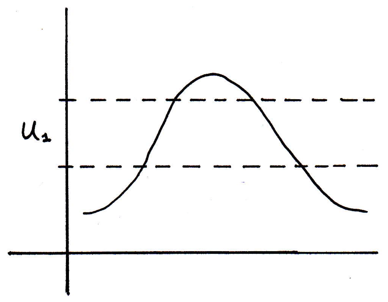
  What is the inverse image of $U_1$ for the figure above? Well, it's the set of all points that get mapped into $U_1$. We can figure that out by just looking at what gets mapped in there. What gets mapped into $U_1$? Well, it looks like two intervals:

  

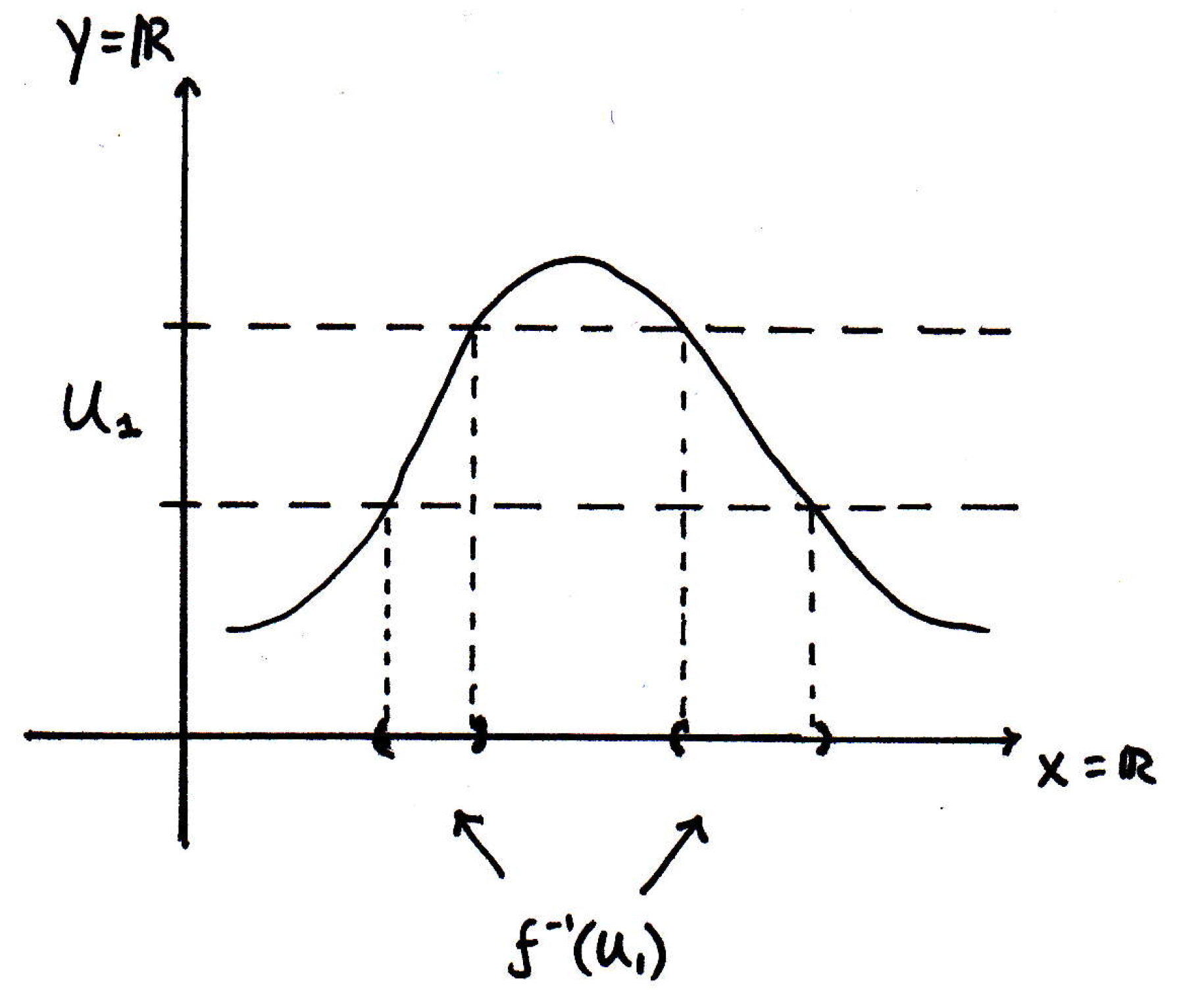
  Note that the sets on the $X$-axis are open are they not? So $f^{-1}(U)$ consists of those two sets. We see that the sets on the $X$-axis do not contain their endpoints because how we've drawn $U_1$ does not contain its endpoints either. Maybe we consider another open set $U_2\subset Y$:

  

  What will the inverse image of $U_2$ be?

  

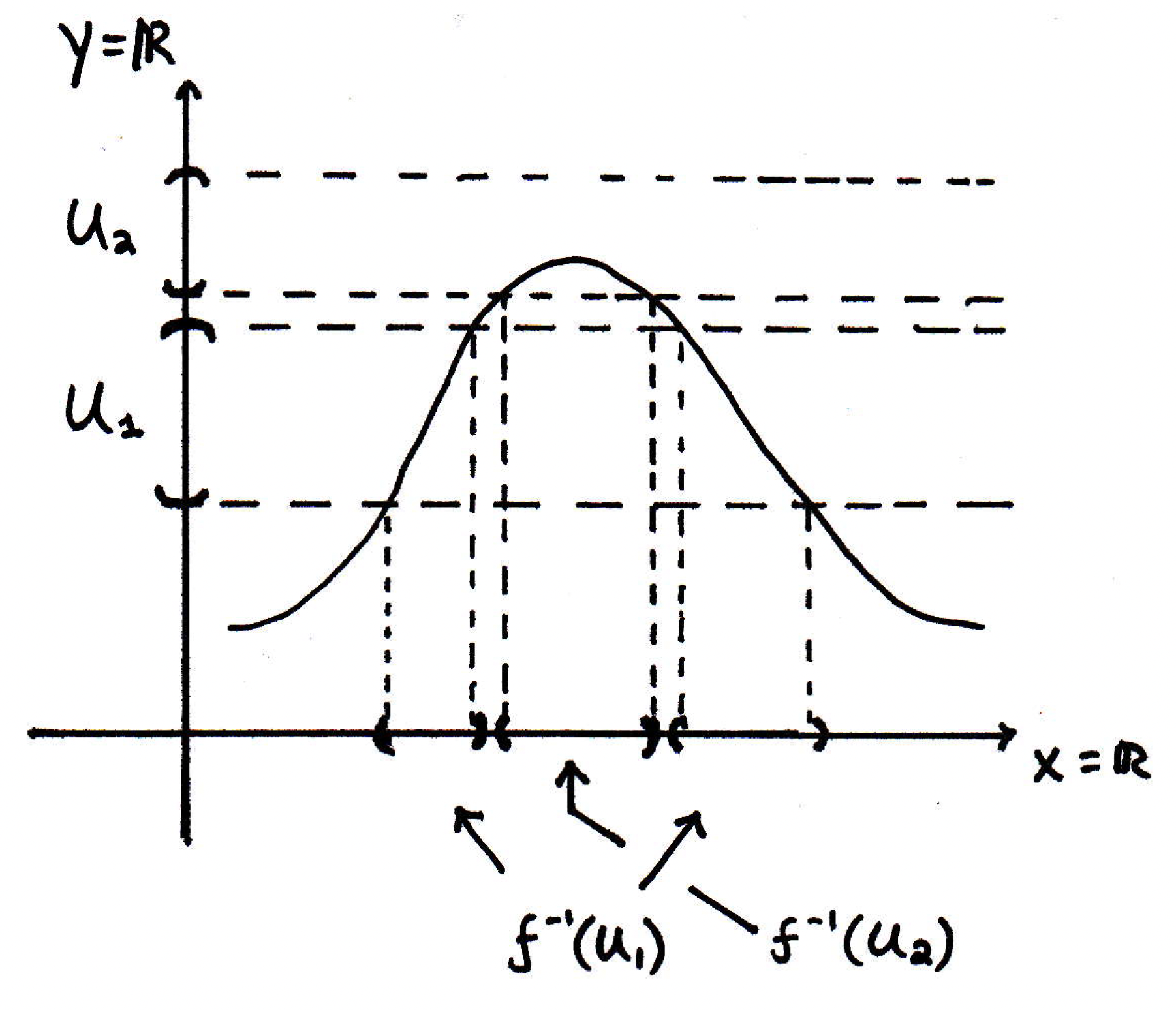
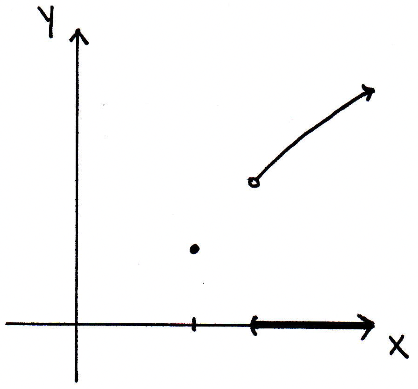
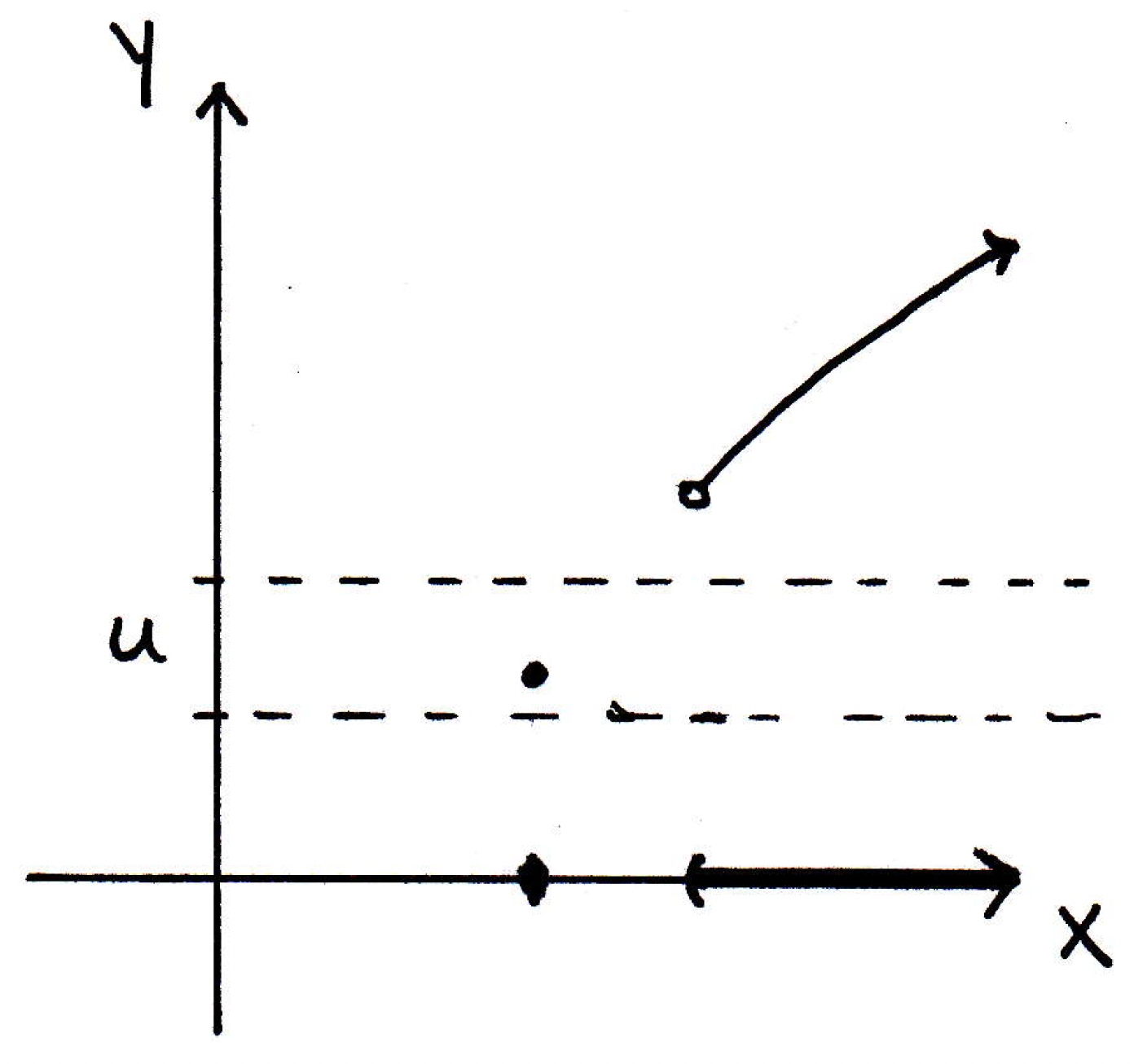
  Notice that there no points get mapped to above the curve in $U_2$, but there are points that get mapped to in the indicated region. So the inverse image of any open set is open so long as the function is continuous. What would go wrong if the function were not continuous? Suppose we have the following function:

  

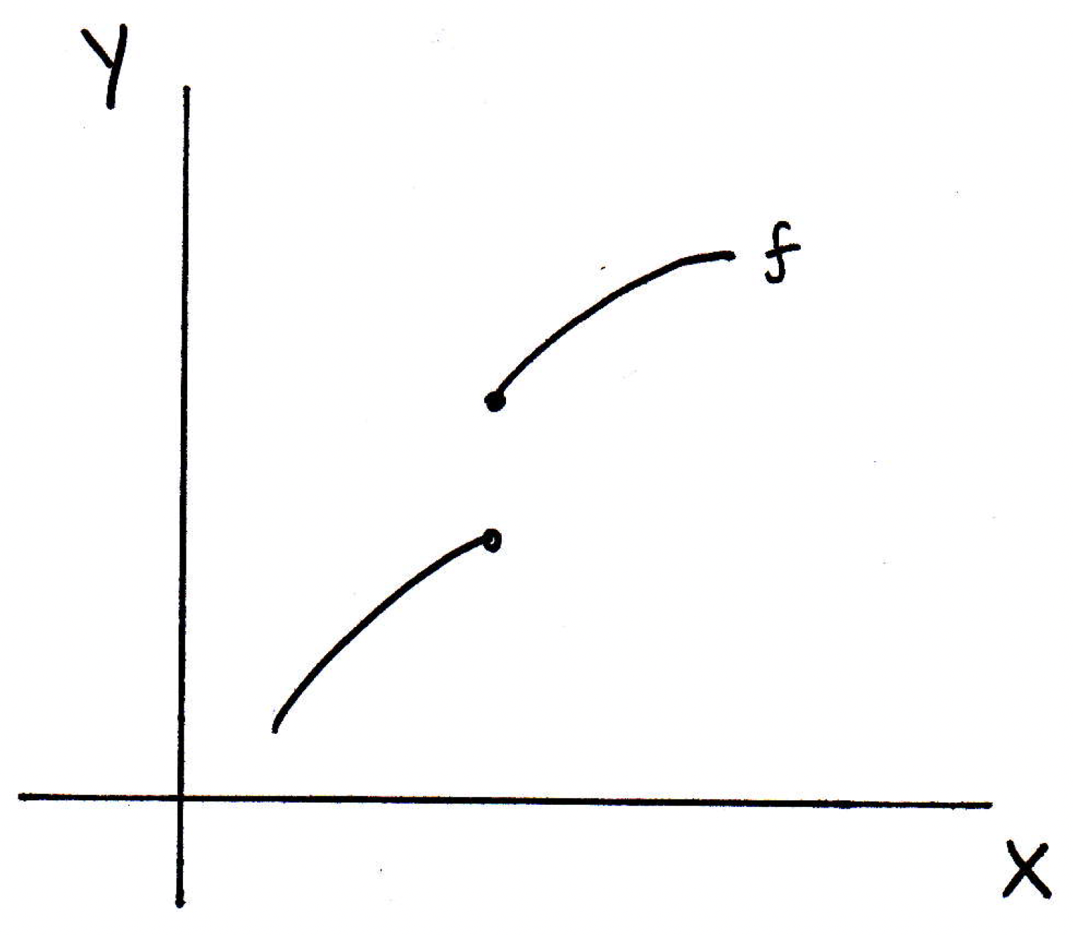
  Can you show me an open set in $Y$ for the function above whose inverse image is not open in $X$? How about an open set that encloses the bolded dot but not the open one? How about the following:

  

  We see that $f^{-1}(U)$ is actually not open. We have a half-open interval. Since we found just one open set in $Y$ whose inverse image was not open, we know the function $f$ pictured above is not continuous.

  Maybe we consider a function $f\colon E\to Y$, where $E$ is not the whole real line but just some subset of it (in the picture below the subset $E$ is just the point on the $X$-axis along with the open interval):

  

  Is the function above continuous? Yes. The only place where we worry about it not being continuous is at the single point (let's call it $p$) off to the left when we are using the $\epsilon$-$\delta$ definition or if you use the limit definition. There's only one sequence that converges to the point $p$ on the $X$-axis, namely $\{p,p,p,\ldots\}$, and the limit of the images of this sequence is $p$, and $f(\lim_{n\to\infty} p_n)=f(p)$ so it satisfies the sequence characterization of continuity. Is it the case here that the inverse image of open sets is open? We might be worried about the following set:

  

  What's $f^{-1}(U)$ for the identified open set $U$ above? It's just the point on the $X$-axis. Is this a problem? No, why not? The inverse image is just a single point, but this point is open in $E$. Why? Because there is a ball around that point in $E$, and the ball only contains that one point so that point by itself is open in $E$.

  So our pictures and example problems jibe with the definition of continuity we have given. Let's now try the proof.

• Restatement of theorem (as seen in [17]): A mapping $f$ of a metric space $X$ into a metric space $Y$ is continuous on $X$ if and only if $f^{-1}(U)$ is open in $X$ for every open st $U$ in $Y$.

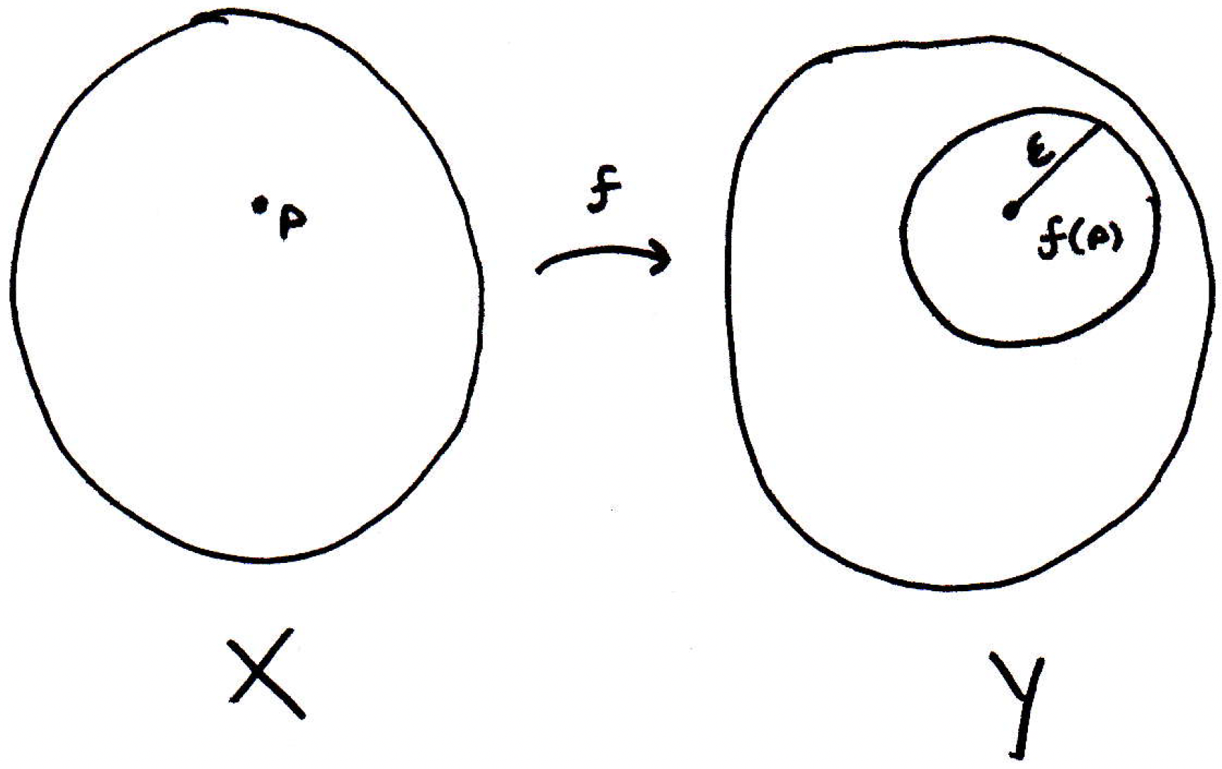
• Forward direction (proof): Let's remind ourselves what it means for a function to be continuous. What it means for a function to be continuous is no matter which point you are at in the codomain, let's say we pick $p$ in the domain and $f(p)$ in the codomain, then you draw an $\epsilon$-ball around $f(p)$, and there is a corresponding $\delta$-ball in the domain whose image is mapped completely into the $\epsilon$-ball. That's the $\epsilon$-$\delta$ definition of continuity. So we'll be able to use that fact if we need it.

  Now, what's our goal in this part of the proof? We are proving the forward direction which means we are assuming that $f\colon X\to Y$ is continuous on $X$ (i.e., for every point in $X$). So the goal, assuming continuity of $f$, is to show that the inverse image of open sets is open. So we should start with an arbitrary open set $U$ in $Y$. Maybe we have a picture that looks like the following:

  

  Our goal, in fact, is to show that the inverse image of $U$ or $f^{-1}(U)$ (i.e., the set of all points in $X$ which get mapped into $U$) is also open in $X$. We have no idea what the inverse image of $U$ looks like, but maybe it looks something like the following:

  

  Who knows whether or not the blobs in $X$ pictured above are open? The two blobs together form $f^{-1}(U)$. How do we show $f^{-1}(U)$ is open? How do we show any set is open? Pick a point inside of $f^{-1}(U)$, say $x$:

  

  What do we do with this point $x$? We want to show that $x$ is an interior point. How do we show that $x$ is an interior point of $f^{-1}(U)$? There's a ball around $x$ whose images lie completely within $U$. But why is that? Why is there a tiny little ball around $x$ whose image lies completely in the set $U$? Because $f$ is continuous! What does that have to do with it? Let's consider the image of our point $x$ in $U$:

  

  Why should there be a ball around $f(x)$? Because $U$ is open. Good. So that means $f(x)$ is interior of $U$ so that's some ball of radius $\epsilon$. So let's draw an $\epsilon$-ball around $f(x)$ to represent this:

  

  Now, because of continuity, there's a $\delta$-ball around $x$:

  

  What's true about the $\delta$-ball around $x$? Its image ``blob'' lies completely in the $\epsilon$-ball:

  

  Since this blob lies completely in the $\epsilon$-ball, then it lies completely within $U$. Let's write out explicitly what we have done in our picture(s).

  Given $U$ open in $Y$, consider $x\in f^{-1}(U)$. We will show $x$ is an interior point of $f^{-1}(U)$. Note $f(x)\in U$, where $U$ is open. Thus, there exists an $\epsilon$-ball $N_\epsilon(f(x))\subset U$. By continuity, there exists a $\delta$-ball $N_\delta(x)$ that maps into $N_\epsilon(f(x))\subset U$. Thus, $N_\delta(x)\subset f^{-1}(U)$. So $x$ is an interior point of $f^{-1}(U)$, as desired, thus concluding the proof of the forward direction of the theorem.

• Backward direction (proof): For the reverse direction, we want to assume that inverse images of open sets are open. And we want to show that, in fact, the function is continuous, and we'll use the $\epsilon$-$\delta$ definition. So how do we do that? Well, start by fixing some $p$ in $X$ no matter which one. (We don't care because this will be a general argument.)

  Fix $p\in X$, and pick some $\epsilon>0$. To show continuity, we want to show that for every $\epsilon>0$ there is a $\delta>0$ such that blah blah blah. So our job is to find a $\delta>0$. That's our goal. Now, you will hopefully use the idea that inverse images of open sets are open (otherwise there would be little sense in claiming the concepts are equivalent). How will we use this idea? Let's draw a picture of the starting situation, where a $p\in X$ has been fixed:

  

  Now, just like before, we'll start off by looking at $f(p)\in Y$:

  

  We'll take an $\epsilon$-ball around $f(p)$:

  

  Our job here is to find a $\delta$-ball around $p$ such that the $\delta$-ball maps completely into the $\epsilon$-ball. Now, the inverse image of open sets is open. Is there an open set on which we can use that fact to our advantage? How about the $\epsilon$-ball? It's an open set. Thus, its inverse image, whatever it is, could look very strange:

  

  It may be helpful to introduce some notation here: Let the $\epsilon$-ball around $f(p)$ be denoted by $B$, and by hypothesis, the inverse image of $B$ or $f^{-1}(B)$ is open in $X$:

  

  Why does that mean there is a $\delta$-ball that maps completely into that $\epsilon$-ball? Since $f^{-1}(B)$ is open, and $p$ lives in the inverse image of $B$, what can we say? We know $f^{-1}(B)$ maps onto the $\epsilon$-ball. The point $p$ is interior to the open set $f^{-1}(B)$ and must therefore have a ball around it. And we'll call the radius of this ball $\delta$, and that will be the $\delta$ we want to use:

  

  Let's try to formalize what we've communicated with pictures above.

  Let $B$ be an $\epsilon$-ball about $f(p)$ in $Y$. Then $p\in f^{-1}(B)$, which is open by assumption. Since $p$ is an interior point of $f^{-1}(B)$, there exists some ball $N_\delta(p)$ that lies completely within $f^{-1}(B)$. This $\delta$ has the required property. Why? It is certainly true that if you are within this $\delta$-ball then the image lies in the $\epsilon$-ball. Why? Because the $\delta$-ball lies in the inverse image of $B$, the $\epsilon$-ball. In summary, the chosen $\delta$ has the required property that ensures $f(N_\delta(p))\subset B$, as desired. Thus, $f$ is continuous.

  As a side note, it should be observed that in the picture(s) above, the $\epsilon$-ball could very will be partially outside of $Y$, where there would then be no preimage for part of it. But that is fine. We're verifying whether or not our function $f$ is continuous at $p\in X$. So we'll be looking at some $f(p)$. Thus, at the very least, the point $f(p)$ will have a preimage. But we don't necessarily know that anything around it has a preimage. It could be the case that the entire blob pictured above in $X$ gets mapped to the single point $f(p)$. That's fine. But then what does an open set around $f(p)$ look like? It will be a ball, but the only thing it will have in its preimage will be that blob.

  Let's now see why this characterization of continuity is very useful.

• Continuity with compositions (see [17]): Consider the continuous functions $f\colon X\to Y$ and $g\colon Y\to Z$ or simply $X\stackrel{f}{\to} Y\stackrel{g}{\to} Z$. The composition of $f$ and $g$ is then continuous; that is, $g\circ f$ is continuous.

  Rudin proves this using the $\epsilon$-$\delta$ definition, but we can have more fun with it now given the definition of continuity involving open sets. So we can use the $\epsilon$-$\delta$ definition if we like, but it's messier than it needs to be. Let's think about this in terms of the open set characterization of continuity.

  If we want to show the composition $X\stackrel{f}{\to} Y\stackrel{g}{\to} Z$ is continuous, where we do $f$ first and then $g$, all we have to do is show that the inverse image of an open set in $Z$ is open in $X$. What should we do? Given $U$ open in $Z$, $g^{-1}(U)$ is open in $Y$ since $g$ is continuous. Then $f^{-1}(g^{-1}(U))$ is open in $X$ since $f$ is continuous. But this is just $(g\circ f)^{-1}(U)$, which is thus open and what we wanted to show, thus concluding the proof.

• Another consequence (concerning closed sets): If the inverse image of open sets is open, what is likely to be the inverse image of closed sets? A closed set. Why? By taking complements. Here's the theorem:

  The function $f\colon X\to Y$ is continuous if and only if for all closed $K\in Y$ then $f^{-1}(K)$ is closed in $X$.

  The proof idea is as follows: If we look at $f^{-1}(K)$ and $f^{-1}(K^c)$, what might be their relationship? It's the set of all things that are mapped into $K$ (i.e., $f^{-1}(K)$) and the set of all things that are mapped into the complement of $K$ (i.e., $f^{-1}(K^c)$). Could they contain anything in common? No, so they're disjoint. Do they contain everything? Yes, they do. So, in fact, we have $f^{-1}(K)=[f^{-1}(K^c)]^c$.

  So if we use our original idea, where we know that $K$ is closed, then we know $K^c$ is open, and the inverse image of an open set is open, and the complement of that is closed. The following visualization may help:

  $$\underbrace{[\underbrace{f^{-1}(\underbrace{(\underbrace{K}_\text{closed})^c}_{\text{open}})}_{\text{open}}]^c}_{\text{closed}}=\underbrace{f^{-1}(K)}_{\text{closed}}.$$

  That's a nice, easy consequence.

• Preservation of compactness for continuous functions: Continuous functions have the curious property that they preserve limits, but they also preserve compactness. Here's a theorem (see [17]): If $f\colon X\to Y$ is continuous and $X$ is compact, then $f(X)$ is compact.

  In other words, if the domain is small, if that space $X$ is small in some sense (recall compact means a set is small in a way, and it's the next best thing to being finite), then its image can't be too big. That's basically what this theorem is saying. Let's give a proof and a quite nice one at that. Consider the space $X$ getting mapped into $Y$ in the following way:

  

  Now, suppose the rest of $X$, that is $X\setminus\{x_1,x_2,x_3,J\}$, gets mapped to just a subset of $Y$, not necessarily all of $Y$:

  

  The claim is that the image on the right-hand side (i.e., $f(X)$) is compact if $X$ is compact. So how do you show that a set is compact? Take an open cover of the creature $f(X)$ and show it has a finite subcover. So let's take an open cover of $f(X)$, where there may be infinitely many such open sets involved in the open cover:

  

  Let $\{V_\alpha\}$ denote the cover sets that cover $f(X)$. Now what? Well, $f$ is continuous; thus, what's really useful here is the open set characterization of continuity. How can that be of use here? Well, this characterization tells us that each of the sets $f^{-1}(V_\alpha)$ is open; hence, we'll get a bunch of open sets $f^{-1}(V_\alpha)$ covering the domain in some fashion:

  

  Now, since $X$ is compact, there exists a finite subcover of $X$; that is, there are finitely many indices, say $\alpha_1,\ldots,\alpha_n$, such that

  $$X\subset f^{-1}(V_{\alpha_1})\cup\cdots\cup f^{-1}(V_{\alpha_n}).$$

  Then $V_{\alpha_1},\ldots,V_{\alpha_n}$ cover $f(X)$. Why? Well, that's just what it means. The inverse image covers $X$ then all the points are in some inverse image. Therefore, applying $f$ to those points puts them in $\{V_\alpha\}$ which covers $f(X)$. More concretely, if $x\in f^{-1}(V_\alpha)$, then $x$ is the inverse image of some point. So $f(x)\in V_\alpha$.

• Remarks following theorem: This should be somewhat surprising. You have a compact set, and its image has to be compact. Recall what the theorem we just proved is saying: If the domain is small (i.e., if $X$ is compact), then the image of our continuous function also has to be small (i.e., $f(X)$ is compact). We might think, in the context of the real numbers, of trying to map an interval onto the whole line. If we consider an interval like $(0,1)$, which is not a compact set, then we can imagine mapping it onto $\R$ (i.e., we essentially stretch the interval $(0,1)$ to cover all of $\R$). In particular, consider $\tan x$, which is continuous on $(-\pi/2,\pi/2)$ and maps onto $\R$. With only a slight modification, we could consider the function $\phi(x)=\tan(\pi(x-\frac{1}{2}))$. Then $\phi$ is mapping $(0,1)$ onto $\R$. In other words, the image of an intuitively small set such as $(0,1)$ can be made to be extremely large such as all of $\R$, as with the case of $\phi$. (Note: This answer on MSE has a better example of a direct map that stretches the unit interval $(0,1)$ onto $\R$.)

  Now, recall that $[a,b]$ is a compact set. So what the theorem we just proved tells us is that it is not possible to map something like $[0,1]$ onto $\R$ if $f$ is continuous. That's impossible because the endpoints have to go somewhere basically.

• Corollary about boundedness (see [17]): If $\mathbf{f}$ is a continuous mapping of a compact metric space $X$ into $\R^k$, then $\mathbf{f}(X)$ is closed and bounded. Thus, $\mathbf{f}$ is bounded.

  Why is the above true? Well, the image $\mathbf{f}(X)$ has to be compact, and in $\R^k$, by the Heine-Borel theorem, it has to be closed and bounded.

• Corollary about obtaining a maximum and minimum (see [17]): Let $X$ be a compact metric space. Then the continuous function $f\colon X\to\R$ achieves its maximum and minimum.

  We use this fact all the time in single- and multivariable calculus when doing optimization problems. In single variable, we are mapping intervals to intervals. In multivariable, we are mapping discs, balls, etc., to other discs, balls, etc. If the intervals, discs, balls, etc., that we are mapping from are compact (bear in mind our mapping is continuous here), then the mapping must achieve its maximum and minimum. Why? Well, its image has to be closed and its image has to be bounded. Its image, being bounded, means it has a supremum and an infimum. Being closed, it means it must contain its supremum and infimum. Done. This is an amazing fact.

• Corollary concerning bijections (see [17]): Let $f\colon X\to Y$ be a bijective mapping (i.e., one-to-one and onto) that is continuous and $X$ is compact. Then $f^{-1}$ is continuous.

  In general, when we have a bijection, we have a one-to-one correspondence, and we can talk about the inverse function because every point has an inverse, a unique inverse. And you might worry that if the forward direction (i.e, mapping $X$ into $Y$) is continuous, then is it necessarily true that the backward direction is continuous as well? The answer is no, not necessarily. But if $X$ is compact, then the forward direction being continuous, in fact, implies that the backward direction is continuous too, which is rather amazing. Let's prove this.

  To show an inverse image is continuous for an inverse function, what you're really trying to show is that if you take an open set in $X$, then the inverse of the inverse, which is going forward, is open in $Y$. (That's the inverse image of the inverse function. It's going forwards from $X$ into $Y$.) Let $U$ be open in $X$. Then $U^c$ is closed. Since $U^c$ is closed, we can use the closed set characterization of continuity as follows: the set $U^c$ is closed in a compact set $X$. Thus, $U^c$ is compact. But if $U^c$ is compact, then its image $f(U^c)$ is compact. But if its image is compact, then it has to be closed. Thus, $f(U)$ is open, which is enough to show that the inverse function is continuous.

• Remark about homeomorphisms: A bijective function that is also bicontinuous is sometimes called a homeomorphism. What it means is that the domain and codomain are topologically equivalent.