8 - Cantor diagonalization and metric spaces

Where we left off last time

Last time we talked a lot about how to count; in particular, we started talking about the size of a set. What does it mean for two sets to have the same size? We agreed that two sets will be deemed to have the same size if we can put those two sets into a one-to-one correspondence with each other. So, in fact, when we count, this is all we are doing. We are actually putting the numbers from 1 through 8, for instance, into one-to-one correspondence with the people in the first row. There are many ways that could be done. I could have done it in a different order, but it doesn't matter. I just need some or one correspondence to say that the numbers 1 through 8 have the same size as the set of people in the first row. Once we had that notion we said that's what it means to count. So we could talk about the size of a set. We could say there are 8 people in the first row because I've just put this set of people in the first row into one-to-one correspondence with the first 8 natural numbers. Then we began to ask about infinite sets. What about sets that have more than a finite number of things in them in some sense? The natural numbers served as an example. We showed that $\N$ is, in fact, an infinite set, which wasn't necessarily obvious because there might secretly have been a one-to-one correspondence between the natural numbers and maybe just the first 8 natural numbers perhaps. But we showed that if there were a one-to-one correspondence for the first 8 numbers, then there would have been one for the first 7. And if there were one for the first 7, then there would have been one for the first 6 and so forth. Then basically that would bring us back to the base case of an induction. And the set of all natural numbers is not in one-to-one correspondence with a set with a single element, as shown in the base case. So we decided to call any set that had the same size or cardinality as $\N$ countable, and we showed last time that $\Q$ is countable. Today we will show more results about countability and uncountability. We will also look at why a set and its power set must have different cardinalities. Then we will start talking about metric spaces.

Recalling the countability proof for Q

Last time we showed that the set of all rational numbers is countable, but there was something that that proof, if you recall how that proof went, we said we could certainly write down all the rationals in a sort of array, namely something like the following:

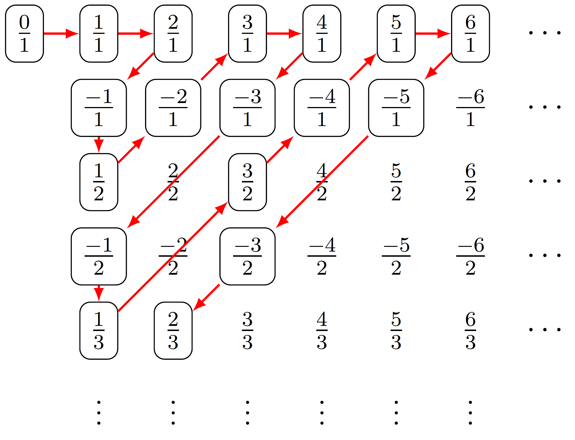
So we said the rationals will be countable if we can list them in some order as a sequence, and of course the problem is with the array that we had we need to find a way to wind our way through this array and hit every fraction. Now, what would be wrong with just going down the first row in the list? We'd never get to the second row. This would just show that the first row is countable. But the way we wind through as illustrated above fixes this problem. So that was the argument for the countability of $\Q$. But I claim that the same argument is, in fact, the proof for another theorem. What we just did with our winding argument is very general so let's see if we can get as much mileage out of it as possible.

Different theorems to prove concerning countability

What are some different theorems to prove concerning countability?

• The countable union of countable sets is countable: This is one of the best ways to show that a set is countable — you write the set in question as a countable union of countable sets. Why is the winding argument for the countability of $\Q$, illustrated above, virtually the same proof for this statement? Well, let's just say each set $A_1$, $A_2$, $A_3$, $A_4$, $A_5$, ... is countable, where this collection is countable because I've indexed the sets using the natural numbers. So if each set is countable, then its members can be listed in a sequence. Then we can write

  $$\begin{align*} A_1&=\{a_{11}, a_{12},a_{13},a_{14},a_{15},a_{16}\ldots\}\\[1em] A_2&=\{a_{21}, a_{22},a_{23},a_{24},a_{25},a_{26}\ldots\}\\[1em] A_3&=\{a_{31}, a_{32},a_{33},a_{34},a_{35},a_{36}\ldots\}\\[1em] A_4&=\{a_{41}, a_{42},a_{43},a_{44},a_{45},a_{46}\ldots\}\\[1em] A_5&=\{a_{41}, a_{42},a_{43},a_{44},a_{45},a_{56}\ldots\}\\[1em] \vdots&{}\qquad\qquad\vdots \end{align*}$$

  Now, can you suggest a way for me to show that everything in the union of the sets listed above is countable? We could zigzag our way through the array hinted at above as follows:

  

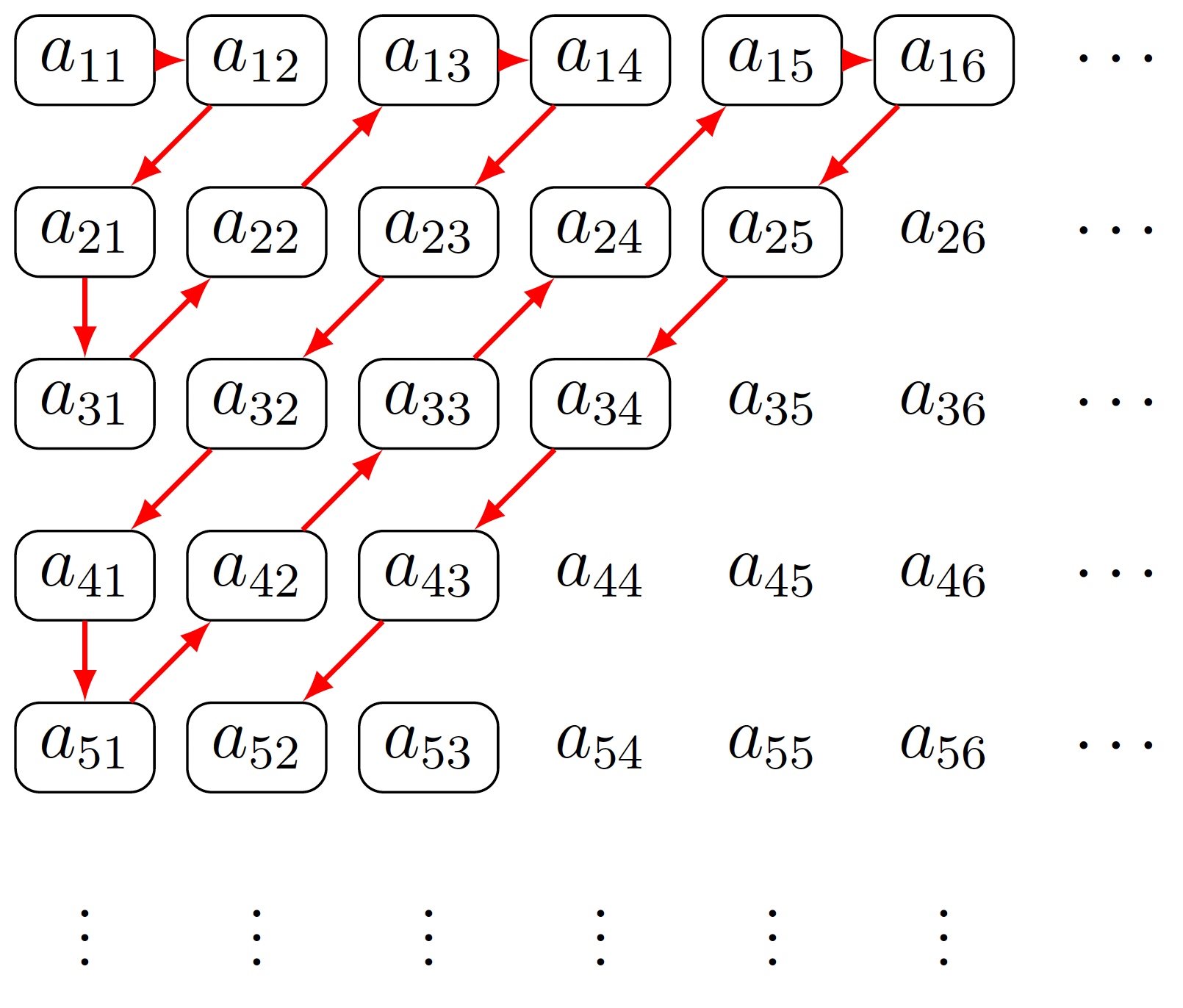
  In this way I get a listing:

  $$\begin{array}{ccc} \text{From}\ \N & {} & \text{From Array}\\ \hline 1&\mapsto& a_{11}\\[1em] 2&\mapsto& a_{12}\\[1em] 3&\mapsto& a_{21}\\[1em] 4&\mapsto& a_{31}\\[1em] 5&\mapsto& a_{22}\\[1em] 6&\mapsto& a_{13}\\[1em] 7&\mapsto& a_{14}\\[1em] 8&\mapsto& a_{23}\\[1em] \vdots&\;\vdots&\vdots \end{array}$$

  An objection may be that a particular element $a_{ij}$ lives in more than one set (maybe many sets). So I would have a listing, but it might list something many times which is not what we want. So what can we do? One way of thinking about this is similar to the rationals where we were just picking equivalence class representatives but not more than one equivalence class member (recall equivalence class representatives were depicted with bubbles around them as all elements $a_{ij}$ are above). If something is already in the set, then you could simply skip over it. Another way of thinking about this is you could just show that this is true for any array and recall the theorem that says that any infinite subset of a countable subset must be countable. So if we just look at all the elements in the zigzag above, some of them may be repeated more than once, but if we take a subset where everything is only chosen once, then such a set is an infinite subset of a countable set and thus countable.

  In sum, we see that if $A_1$, $A_2$, $A_3$,\ldots are countable sets, then $\displaystyle\bigcup_{i=1}^\infty A_i$ is countable. It should be noted that whenever you are talking about an arbitrary union that is not necessarily countable, then we use a different notation. (As a side note, observe that if the collection of sets is not necessarily countable then you cannot use natural numbers as an index because that would make the reader think that you are talking about a countable collection). So if you want to refer to something that is not necessarily countable, the traditional way to do that is to give the subscript $\alpha$ or a Greek letter and then you union over all $\alpha$ in some index set $J$:

  $$\bigcup_{\alpha\in J}A_\alpha.$$

  So use the notation $\bigcup_{\alpha\in J}A_\alpha$ for a possibly uncountable collection, where $J$ is an index set.

• Modification of theorem statement: In the statement of the theorem "the countable union of countable sets is countable" there was a question as to what happens if one of the sets is finite. Well, what could we do? You could imagine that if one of the sets $A_i$ is finite, then its listing of elements simply terminates, and the $i$th row of the zigzag argument will have empty row entries upon termination. (You could think of it as leaving behind an empty block or row segment.) And again what you are looking at is a subset consisting of the nonempty blocks of an array that is countable. So the theorem "the countable union of countable sets is countable" is, in fact, true if you replace all of the words "countable" here by "at most countable," where at most countable includes being finite. So if you want to take the finite union of countable sets, then that is still countable or finite. Or the finite union of finite sets is finite. So that is also true as well.

• Example involving computer programs: Consider the set of computer programs. What is a computer program? How do you normally code up a program? You code it up using some language, which consists of letters or symbols. And what do you do with those symbols? You string them together. So a computer program could be thought of as a collection of symbols. Each program is a collection of symbols. How many symbols? Finitely many. Each of those symbols could have how many possibilities? Finitely many if it's an alphabet of some kind. So each program is finite. What about the collection of all computer programs? It's the union of all 0-character programs, 1-character programs, 2-character programs, 3-character programs, etc. So, in fact, what we have here is the fact that the set of all computer programs is countable. (It won't be finite because there are countably many unions and they're nonempty.) Why is that an amazing fact? Recall that $\R$ is not countable. So we say that $\R$ is uncountable (i.e., infinite and not countable). So $\R$ is uncountable yet the set of all computer programs is countable. What does this mean? This means that there are some real numbers that can never be the output of a computer program. So let's call a real number computable if through some algorithm you can compute its decimal expansion up to a specified number of places. (So if you input a number $k$ and the program outputs the $k$th places of the real number. That's one of these computer programs.) So there are some real numbers that are not computable (i.e., cannot be the output of a computer program).

  On your homework you are asked to show that the set of algebraic numbers is countable. An algebraic number means it can appear as a root of a polynomial with integer coefficients, and it uses a very similar method. You think about what kinds of polynomials you could have and those are specified by the coefficients. And how long could a polynomial be? Well it could be quite long, many many, many terms but finitely many terms.

Follow up on Cantor's diagonalization argument for the real numbers

Follow up on Cantor's diagonalization argument that showed the real numbers to be uncountable. (Note that this is not the zigzag argument we used earlier for $\Q$ and the theorem concerning a countable collection of countable sets.)

• Power sets: Cantor's argument is an example of something even more general. So a general fact is a theorem about power sets. Now, given a set $A$, the power set $2^A$ is the set of all subsets of $A$. If $A=\{\blacklozenge,\Box,\triangle\}$, then $D=\{\blacklozenge,\triangle\}$ and $E=\{\triangle\}$ and $\emptyset$ are all subsets of $A$ or elements of $2^A$, and there are others as well. How many subsets are there of $A$? There are $2^3=8$. Is that a coincidence? No. Why? The set $D$ corresponds to a particular binary number, namely 101, where a 1 indicates that the particular element in $D$ is also in $A$ while a 0 indicates this is not so. (Of course, for such a binary structure to have much meaning, we need to say that the elements of the set $D$ are ordered even though we generally do not care about order for set elements.) So we can write $D\mapsto 101$, $E\mapsto 001$, and $\emptyset\mapsto 000$, and so forth. Well, there are only 2 possibilities for each binary string entry, and there are 3 entries in total due to the number of elements in $A$. Thus, in this case, the total number of distinct binary numbers is $2\cdot2\cdot2=2^3$. In general, we have $2^{|A|}$ subsets of $A$. This is the fundamental idea that is used in proving Cantor's theorem.

• Cantor's theorem (diagonal argument): For any set $A$ (so $A$ could be hugely uncountable or whatever we want essentially), we cannot put $A$ into one-to-one correspondence with its power set; that is, $A\not\sim2^A$. Suppose there does exist a bijection $f\colon A\twoheadrightarrow2^A$. So this function $f$ should take something in $A$, like $\Box$, and it will output a subset like $D$ or $E$ above or $\emptyset$. What this means is that $a\mapsto f(a)$, which is a subset of $A$. It might be something like $\Box\mapsto\{\Box,\triangle\}$. Since we have a bijection, we should try to describe it. How will this proof be similar to the given proof before concerning the uncountability of $\R$?

  Maybe we take $a\in A$ and associate with that element $f(a)$ which is in the power set. We could write out the following (It's important to note here that we are not necessarily, and often not, dealing with countable sets. We don't want to represent things as a list, especially not a sequence, since that gives the impression that we are dealing with something countable, but there's little chance to avoid this way of thinking in terms of just charting out our ideas.):

  $$\begin{array}{ccc} a\in A & {} & f(a)\in 2^A\\ \hline \blacklozenge&\mapsto& \underbrace{\left\{\begin{matrix}\triangle&\Box&\blacklozenge\\ \diamond&\star&{}\end{matrix}\right\}}_{\substack{\text{jumbled elements}\\\text{of $A$ not in a list}}}\\[5em] \diamond&\mapsto& \underbrace{\left\{\begin{matrix}\triangle&\star&{}\\ \blacklozenge&\blacktriangleleft&\spadesuit\end{matrix}\right\}}_{\substack{\text{jumbled elements}\\\text{of $A$ not in a list}}}\\[5em] \star&\mapsto& \underbrace{\left\{\begin{matrix}\star&\spadesuit&{}\\ \clubsuit&\Box&{}\end{matrix}\right\}}_{\substack{\text{jumbled elements}\\\text{of $A$ not in a list}}} \end{array}$$

  The above is not a list even though it looks like it. What's going to be the analog of the diagonal argument that we used for $\R$? We constructed a decimal number in the right hand number by appealing to each sequence of numbers in the table and changing the number if appropriate, thus ensuring we never ended up with a number in the table. What's going to play that role here? I want to show that there is no bijection $A\sim2^A$ by showing that there is a subset that cannot be on the right side in the scheme presented above. And I'm going to do this by making this subset differ from every possible thing on the right hand side. How am I going to make it different? In what place? Well, given everything in the set $A$, we can specify a subset of $A$ by deciding whether or not an element is in it.

  I want to construct a new set which differs from everything in the list

  $$\begin{array}{ccc} \text{Subset of $A$} & {} & \text{Binary representation}\\ \hline D&\mapsto& 101\\[1em] E&\mapsto& 001\\[1em] \emptyset&\mapsto& 000 \end{array}$$

  in the what place? Well, given $A=\{\blacklozenge,\Box,\triangle\}$, maybe we associate with $\blacklozenge$, an element of $A$, the set $D=101$, a subset of $A$. More specifically, given our way of using binary numbers as subset representations, perhaps we make the associations

  $$\blacklozenge\mapsto D=101,\quad \Box\mapsto E=001,\quad \triangle\mapsto \emptyset=000.$$

  We want to construct a set that differs from the "black lozengeth element" of the list in the "black lozengeth place" and differs from the "boxeth element" in the "boxeth" place and differs from the "triangleth element" in the "triangleth place":

  $$\begin{array}{c|ccc} {} & A &= &\{\blacklozenge,\Box,\triangle\}\\ \hline \blacklozenge & D &\mapsto & {{\color{red}{1}}}01\\[1em] \Box & E &\mapsto & 0{{\color{red}{0}}}1\\[1em] \triangle & \emptyset &\mapsto & 00{{\color{red}{0}}} \end{array}$$

  If I were to do this for this particular picture, I'm really interested in constructing a set that's not ${{\color{red}{100}}}$ but ${{\color{red}{011}}}$, and I claim if that's the case then ${{\color{red}{011}}}$ is a new set, namely $\Box$ and $\triangle$, that can't be on my list anywhere. That's the basic idea. Recall the association we were starting to set up:

  $$\begin{array}{cccr} a\in A & {} & f(a)\in 2^A & a\in f(a)\,?\\ \hline \blacklozenge&\mapsto& \underbrace{\left\{\begin{matrix}\triangle&\Box&\blacklozenge\\ \diamond&\star&{}\end{matrix}\right\}}_{\substack{\text{jumbled elements}\\\text{of $A$ not in a list}}} & \text{Yes}, \blacklozenge\in f(a)\\[5em] \diamond&\mapsto& \underbrace{\left\{\begin{matrix}\triangle&\star&{}\\ \blacklozenge&\blacktriangleleft&\spadesuit\end{matrix}\right\}}_{\substack{\text{jumbled elements}\\\text{of $A$ not in a list}}}& \text{No}, \diamond\not\in f(a)\\[5em] \star&\mapsto& \underbrace{\left\{\begin{matrix}\star&\spadesuit&{}\\ \clubsuit&\Box&{}\end{matrix}\right\}}_{\substack{\text{jumbled elements}\\\text{of $A$ not in a list}}} & \text{Yes}, \star\in f(a) \end{array}$$

  Based on what we see above, what's the new subset $B$ I would construct? Should we have $\blacklozenge\in B$? No! Should we have $\diamond\in B$? Yes! Should we have $\star\in B$? No! In general, what is the set $B$ going to be? This is how you motivate this construction. (What we want is a subset $B$ that is not in the image of $f$ — it can't be the image of any particular element in $A$.) Let $B=\{a\mid a\not\in f(a)\}$. This is our proposal. Let's see whether or not it's in the image of anything. If $B=f(x)$ for some $x\in A$, what would go wrong? We can modify our previous picture to look as follows:

  $$\begin{array}{cccr} a\in A & {} & f(a)\in 2^A & a\in f(a)\,?\\ \hline \blacklozenge&\stackrel{f}{\mapsto}& \underbrace{\left\{\begin{matrix}\triangle&\Box&\blacklozenge\\ \diamond&\star&{}\end{matrix}\right\}}_{\substack{\text{jumbled elements}\\\text{of $A$ not in a list}}} & \text{Yes}, \blacklozenge\in f(a)\\[5em] \diamond&\stackrel{f}{\mapsto}& \underbrace{\left\{\begin{matrix}\triangle&\star&{}\\ \blacklozenge&\blacktriangleleft&\spadesuit\end{matrix}\right\}}_{\substack{\text{jumbled elements}\\\text{of $A$ not in a list}}}& \text{No}, \diamond\not\in f(a)\\[5em] \star&\stackrel{f}{\mapsto}& \underbrace{\left\{\begin{matrix}\star&\spadesuit&{}\\ \clubsuit&\Box&{}\end{matrix}\right\}}_{\substack{\text{jumbled elements}\\\text{of $A$ not in a list}}} & \text{Yes}, \star\in f(a) \end{array}$$

  So in the picture above, the claim is that the set $B$ is somehow corresponding to some $x$ through $f$. What would we then look at? Well, if $B=f(x)$ for some $x\in A$, then consider $x$. Is $x\in B$? No. Why not? If $x$ were in $B$, then $x$ would not be in $f(x)$. But $x\not\in f(x)$ would contradict the fact that $x\in B$. So it must be the case that $x\not\in B$. But if $x\not\in B$, then $x\in f(x)$. But, by the definition of $B$, this would mean that $x\in B$, contradicting again the assumption that $x\not\in B$. Either way we get a contradiction. So $B$ is not $f(x)$ for any $x\in A$. That's the end. Such a bijection could not have existed. That's the desired contradiction.

Thinking about the power set

What are some useful ways of thinking about the power set?

• Power set of $\R$: What's an example of a power set of $\R$? So what we've learned is that there are many different "sizes" of infinity. There are many cardinalities. For instance, what is a set with cardinality $2^\R$ that has the same cardinality as the power set of the real numbers? Another way to talk about subsets of a set is to associate to each real number a 0 or a 1. What is that? That's just a function $f\colon\R\to\{0,1\}$. Notice that $2^A\sim\bigr\{f\colon A\to\{0,1\}\bigr\}$. This is just by the membership relation. So $2^\R\sim\ \text{all *functions* from}\ \R\to\{0,1\}$. A consequence of this theorem is that there are infinitely many cardinalities. We have the cardinalities,

  $$0,1,2,3,4,\ldots,\aleph_0,\aleph_1,\aleph_2,\ldots,\aleph_\omega,\ldots$$

  where $\aleph_0$ is the first size that is not finite. And then, of course, you can argue that there is a first size that is not $\aleph_0$, and that is called $\aleph_1$, and so on, where the indices for $\aleph$ are indexed by what are called ordinal numbers. The continuum hypothesis is basically the following fact: The cardinality $\aleph_0$ is the cardinality of $\Z$. And the cardinality of the reals, often denoted $\mathfrak{c}$, is often called "the continuum." So you might ask which $\aleph$ is equivalent to $\mathfrak{c}$. So where might $\mathfrak{c}$ belong in this picture? In the continuum hypothesis, the claim or the hypothesis is that $\mathfrak{c}=\aleph_1$. And what's known is that whether the answer is yes or no is not provable within the axioms that we have. It can be taken to be true or false without changing the axioms of ZFC set theory.

Metric spaces

What exactly are metric spaces and why are they useful?

• Introduction: We're going to develop tools that will allow us to work with collections of things that aren't just real numbers. This is why it is important to talk about metric spaces. So what is a metric space? Well, as the name suggests, a space is like a space — it's more than just a set. You could have a set of things, but when you start talking about spaces of things, it kind of implies that there's a notion of what? Space. Big. Small. There's some way to move throughout the space. So this is the idea when we use the word "space" — it is a set that is endowed with "something extra," and often it's a metric. So the idea of a metric is the notion of distance. So how do we measure distance? Now, if you're talking about the real line, then there's a standard way to do that. You can talk about the distance between two points. But you could be talking about other thing. You could be talking about three-dimensional space, you could be talking about spaces of phylogenetic sequences. You give me the genetic code of a human and a rat and a rabbit, and I might want to know which of those genetic codes are closer in some sense. So how do we measure distance? What are we going to mean by that? We could look at $\R^n$ or the set of genome sequences. There are all sorts of sets we could look at.

• Defining a metric: We are going to define a notion of distance, and this notion will be called a metric.

  Metric (definition): A set $X$ is a metric space if there exists a metric (what is a metric? It's a function that takes in pairs of points and returns a nonnegative real number.) $d\colon X\times X\to\R$ such that the following properties are true for all $p,q\in X$:

  1. $d(p,q)\geq0$, where $d(p,q)=0$ if and only if $p=q$\hfill(nonnegativity)
  2. $d(p,q)=d(q,p)$\hfill(symmetry)
  3. $d(p,q)\leq d(p,r)+d(r,q)$ for any $r\in X$\hfill(triangle inequality)

  This seems like a pretty natural notion of distance, but let's see some examples of distances.

• What are some examples of a distance: The first one, of course, is just the notion of absolute value of the difference of two numbers. That's definitely a distance. So our set in this case is $\R$ and the metric is $d(x,y)=|x-y|$. If there's any confusion, then I would specify what the metric is exactly. So here I would write $(\R,d)$ [that is, the metric is a pair; it is $\R$ together with $d$], if there's any confusion. Now, how about $\R^n$ with the distance $d(\overrightarrow{\mathbf{x}},\overrightarrow{\mathbf{y}})=\sqrt{(x_1-y_1)^2+\cdots+(x_n-y_n)^2}$. It's the distance formula. And note that the metric on $\R^n$ is the same as the metric on $\R$ when $n=1$, which can easily be seen by noting that $\R^1=\sqrt{(x_1-y_1)^2}=|x_1-y_1|$. This is known as the Euclidean metric on $\R^n$. Anytime you have a metric on $\R^n$ where the metric is not specified, you may assume that the Euclidean metric is what is being considered. For this reason, this metric is sometimes called "the usual metric," if not otherwise specified. But there are many others. Also in $\R^n$, we could have the distance $d(\overrightarrow{\mathbf{x}},\overrightarrow{\mathbf{y}})=\sum_{i=1}^n |x_i-y_i|$. So the staircase metric gives a different notion of distance than the Euclidean notion. Let's talk about some other spaces than $\R^n$. So you might look at a phylogenetic tree or any tree for that matter (where a tree is a bunch of nodes connected by edges where there are no loops or cycles). Now imagine the figure

  

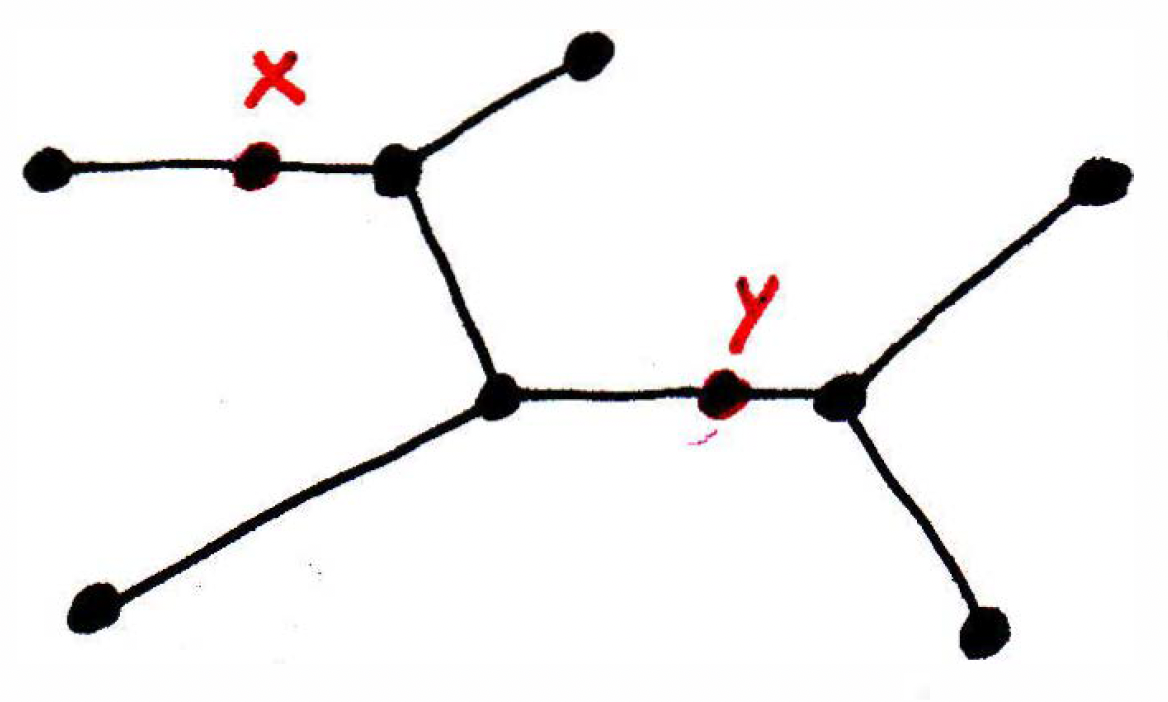
  not as a graph which is basically a discrete object but a continuous object where you could live anywhere along an edge. In the above, let's measure the distance between $x$ and $y$. What would this mean? How would you measure the distance? We could count the number of vertices between $x$ and $y$ in the picture above, but the distance would be 0 if they were on the same edge. (Such an instance is called a pseudometric.) If it were a continuous space, then we could just add up the edge length portions between $x$ and $y$. That's one notion of distance. So this is the tree metric $d_T(x,y)=$ length of the shortest path between $x$ and $y$. (This is well-defined on a tree — there's a shortest path between two vertices, and this path is unique.)

  For another example, suppose $X$ is the set of genome sequences. Right now we'll ignore the possibility that some sequences might have different lengths than others. Imagine you have a bunch of sequences of the same length. So, for instance, one sequence might be

  $$\overrightarrow{\mathbf{x}}=\mathrm{GATTACA},\quad \overrightarrow{\mathbf{y}}=\mathrm{AGATCAT}.$$

  What might be a good notion of distance between $\overrightarrow{\mathbf{x}}$ and $\overrightarrow{\mathbf{y}}$? Let's call the distance $d_G(\overrightarrow{\mathbf{x}},\overrightarrow{\mathbf{y}})$. What's a decent sense of distance? Perhaps the number of differences or letters that are different. Is that a metric? We have to check the three properties. Is it only 0 when they are equal? Yes, good sign. Is it symmetric? Yes. Satisfy the triangle inequality? It actually does!

  Now what about the following: Often you are dealing with a space of functions. You often have functions you are dealing with. Suppose you have two curvy functions. How would you measure the difference between such functions? How would you define the distance between functions $f$ and $g$? There are several different ways, but let's hear some ideas. We could let $d_I(f,g)=\int_a^b|f-g|\,dx$ as long as this is defined between some $a$ and $b$, where maybe we define this for continuous functions on $[a,b]$. That's the space. A space of continuous functions on $[a,b]$, and this is often written $C[a,b]$, where $C$ means the set of continuous functions. Okay, that's definitely one way of doing it. Is it true $d_I(f,g)$ in this case will be 0 when $f=g$? Yes, if $f$ and $g$ are continuous. But if they're not continuous, then we'd have to place functions into equivalence classes possibly.

  We could look at $d(f,g)=\displaystyle\sup_{x\in\R}|f(x)-g(x)|$ so long as we're on the space of continuous bounded functions, which is often denoted $C_b(\R)$. (The maximum may never be achieved, but we will always have a supremum when dealing bounded sets of real numbers.) The distance $d_{\mathrm{sup}}(f,g)=\displaystyle\sup_{x\in\R}|f(x)-g(x)|$ is actually called the supremum distance or "sup norm."

• Some ideas to build upon for next time: In a metric space, one of the most important concepts which helps you get a sense of what the metric is doing is the concept of an open ball. What is an open ball? Well, you think of a ball as a round object, and mathematically that would be the set of all points whose distance is less than or equal to some number (or less than for an open ball). We write $N_r(x)=\{y \mid d(x,y)<r\}$. If you want the closed ball, then it's the same definition except the "$<$" becomes a "$\leq$" and we might notate it by $\overline{N_r(x)}$. Under the Euclidean metric, an open ball would look like what we expect, namely an open ball, whereas for the staircase metric the open ball would look like a diamond. Why are balls going to be important? Well, balls are going to be important because we can use them to define the notion of what it means for things to be close as in a limit point. What does it mean for a point to be a limit point for some set?

• Limit point example 1: Suppose we have the following picture:

  

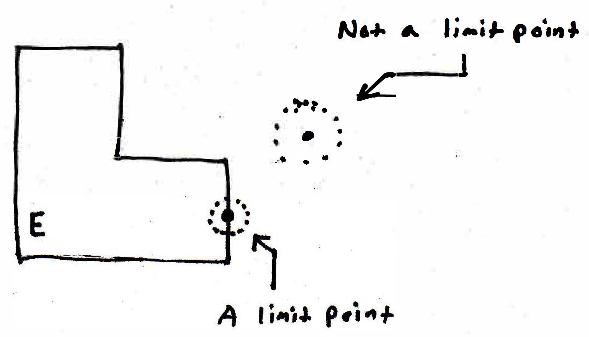
  What does it mean for the point indicated as a limit point to actually be a limit point of the set $E$? What it means is you give me any ball around the indicated point, then no matter what ball I take I will always have points of set $E$ contained within that ball. The other point indicated is not a limit point because there is a ball which does not touch $E$ at all. This motivates the following definition:

  Limit point (definition). Say $p\in X$ is a limit point of $E$, where $E\subseteq X$, if every neighborhood of $p$ contains a point $q\neq p$ such that $q\in E$.

  The next example may help illustrate this definition.

• Limit point example 2: Suppose we have the set of reciprocals, where part of the picture is illustrated below.

  

  It's clear that the reciprocals are clustering around 0, but does this set have a limit point? Yes, we claim 0 is a limit point because any open ball around the set contains a point.