25 - Taylor's theorem

Where we left off last time

What are some applications of the derivative? Where did we leave off last time and where were we going?

• Recap: We have been talking about the derivative. Last time we defined the derivative. We said what it means for a function to be differentiable, which basically means that a certain limit exists. The derivative is the limit of a difference quotient, where the difference quotient represents the slope of a secant line. We say that a function is differentiable at a point $x$ if the limiting slope of a secant line actually exists. We also talked about a very important theorem which basically is the most important theorem when it comes to derivatives. It connects the value of the function to the value of the derivative. It was the mean value theorem. Today we'll see how it's important and talk about a generalization known as Taylor's theorem. (Taylor's theorem is really just a generalization of the mean value theorem.) That will be the first part of this lesson. The second part we will discuss sequences of functions, which is a different topic.

• Taylor's theorem (motivation): Suppose you know something about a function and what it is doing at a particular point. The idea of Taylor's theorem is, well, if you know about what's happening at a point, then you know what's happening near a point, if it's differentiable, if it's twice-differentiable, or if you have a number of derivatives. In the simplest case, suppose we know what a function $f$ is doing at a point $a$, and we want to approximate what's happening near $a$, say at a point $b$. That is, given we know something about $f(a)$, suppose we want to approximate $f(b)$, where $b$ is near $a$.

  Well, the mean value theorem tells us something about $f(b)$ if we know $f(a)$ and the derivative nearby. So the mean value theorem basically says I can figure out what $f(b)$ is if I know $f(a)$ and I know something about the derivative nearby:

  $$f(b)=f(a)+f'(c)(b-a).$$

  Observe how this is a restatement of the mean value theorem. And the thing to notice here is that there is a mysterious point $c$, and all we know about $c$ is that it lives between $a$ and $b$. That is, we have $f(b)=f(a)+f'(c)(b-a)$ for some $c\in(a,b)$. So we have no idea what point $c$ is. The way to think about this is that we will know $f(b)$ if we know $f(a)$ and $f'(c)(b-a)$, a term we have little control over or know much about. What we do know is that this term is something like an error term. It tells us how far off $f(b)$ is from $f(a)$. So we can think of the formulation like so:

  $$f(b)=f(a)+\underbrace{f'(c)(b-a)}_{\substack{\text{"error" term not}\\\text{precisely known}}}.$$

  This "error term" is often not precisely known. But it has something to do with the derivative nearby. So if we can bound the derivative nearby, then maybe we can actually say something about that error. That is one way of thinking about the mean value theorem.

  This actually suggests that we might be able to do better with our approximation. We don't know what $f'$ is doing at $c$. We don't even know where $c$ is. But what if we knew what the derivative was doing at $a$? Then maybe we could do better. This suggests that maybe

  $$f(b)=f(a)+f'(a)(b-a)+\text{error},$$

  where this "error" term is hopefully smaller than the error term before. So this suggests there might be a theorem like this: can we fill in this process where the error terms get smaller and smaller? And the answer is yes. If our function were twice differentiable, then we get $\frac{f"(c)}{2}(b-a)^2$ as our error term, where this $c$ is not the same $c$ as that in the first statement but just some $c\in(a,b)$. Notice that the error term $\frac{f"(c)}{2}(b-a)^2$ is a little bit better than what we originally had because if $b-a$ is really small, then $(b-a)^2$ is really small. But once again, we have no control over where $c$ is. We just know $c\in(a,b)$.

  So this is sort of the direction Taylor's theorem goes in. It gives us some sort of idea of how good this particular error term is. What's the moral of this story? The moral is that if we know a function value $f(a)$ and its derivative $f'(a)$, and we know its second derivative in some neighborhood of $a$, then we will have a good handle on what $f(b)$ is.

  Of course, we could continue the process above. We could say the error term in

  $$f(b)=f(a)+f'(a)(b-a)+\text{error}$$

  is kind of like a second derivative. So maybe if we thrown in a term like $\frac{f"(c)}{2}(b-a)^2$, where $c$ is replaced by $a$ (i.e., we would have$\frac{f"(a)}{2}(b-a)^2$), then we will yet still get a better error term. That's really the direction that Taylor's theorem goes into.

• Taylor's theorem (statement): Generally, if

  $$P_{n-1}(x)=f(a)+f'(a)(x-a)+\frac{f"(a)}{2!}(x-a)^2+\cdots+\frac{f^{(n-1)}(a)}{(n-1)!}(x-a)^{n-1}.$$

  Here's what we should notice: where do the $x$'s appear in the expression above? The first term is just a constant with respect to $x$. There's an $x$ in the next term, an $x^2$ in the following term, and so on. So we see that $P_{n-1}(x)$ is a polynomial in $x$ (or really a polynomial in $x-a$) and its degree is $n-1$. What is the dependence on $a$? To determine the coefficients, note that $f'(a)$ is involved with every single one of them. So $P_{n-1}(x)$ is a polynomial, and it is often called a Taylor polynomial.

• Taylor's theorem (statement): If $f^{(n-1)}$ is continuous on $[a,b]$ and $f^{(n)}$ exists on $(a,b)$, then $P_{n-1}(x)$ approximates $f(x)$, and

  $$f(x)=P_{n-1}(x)+\underbrace{\frac{f^{(n)}(c)}{n!}(x-a)^n}_{\text{error term}},$$

  where $c\in(a,b)$.

  Note that the error term here looks a lot like the terms of the Taylor polynomial except that the $n$th derivative is evaluated somewhere between $a$ and $b$. What does this theorem say in the case that $n=1$? Can we prove this theorem in the case where $n=1$? Yes, what is it? (Note that $P_{1-1}=P_0=f(a)$ when $n=1$.) Well, the function $f$ is just saying "tell me what's going on at $f(a)$," and add what? We'd add $\frac{f'(c)}{1!}(x-a)$. That is, for $n=0$, we should have

  $$f(x)=f(a)+\frac{f'(c)}{1!}(x-a)$$

  Is that true for some $c\in(a,b)$? Yes, by the mean value theorem. When $n=1$, this literally is the mean value theorem. So Taylor's theorem really is just a generalization of the mean value theorem.

  Now, $P_n(x)$ is the "best" approximation of order $n$ at $a$. What do we mean by "best" here? Well, what we mean is we've constructed a polynomial that has all the same value in derivatives up to the $n$th; that is, $P_n(x)$ has the same value of $f', f", f"', f^{(4)},\ldots,f^{(n)}$ at $a$. That is, we have the following correspondence (at $a$):

  $$\begin{matrix} f & f' & f" & f"' & \cdots & f^{(n)}\\[1em] \updownarrow & \updownarrow & \updownarrow & \updownarrow & \cdots & \updownarrow\\[1em] P & P' & P" & P"' & \cdots & P^{(n)} \end{matrix}$$

  So the first derivative of the polynomial and the first derivative of $f$ both have the same value at $a$. Let's just convince ourselves of that. If we look at the polynomial

  $$P_{n-1}(x)=f(a)+f'(a)(x-a)+\frac{f"(a)}{2!}(x-a)^2+\cdots+\frac{f^{(n-1)}(a)}{(n-1)!}(x-a)^{n-1}$$

  at $x=a$, then we see that we have

  $$P_{n-1}(x)=f(a)+\underbrace{f'(a)(x-a)}_{=0}+\underbrace{\frac{f"(a)}{2!}(x-a)^2}_{=0}+\cdots+\underbrace{\frac{f^{(n-1)}(a)}{(n-1)!}(x-a)^{n-1}}_{=0}=f(a)$$

  because all of the other terms go to zero.

  What happens if we take the first derivative of $P_{n-1}(x)$? What happens to the $f(a)$ term? It disappears because the derivative with respect to $x$ is gone. What happens when we take the derivative of $f'(a)(x-a)$ with respect to $x$? We just get $f'(a)\cdot1=f'(a)$. And the rest of the terms have positive powers of $x-a$ in them and hence evaluate to zero at $x=a$. So $(P_{n-1}(x))'=f'(a)$.

  Similarly, if we look at $(P_{n-1}(x))"$, then we have the following:

  $$(P_{n-1}(x))"=\underbrace{f(a)}_{\text{vanishes}}+\underbrace{f'(a)(x-a)}_{\text{vanishes}}+\underbrace{\frac{f"(a)}{2!}(x-a)^2}_{\substack{\text{survives and}\\\text{evaluates to $f"(a)$}}}+\underbrace{\cdots+\frac{f^{(n-1)}(a)}{(n-1)!}(x-a)^{n-1}}_{\text{vanishes}}=f"(a).$$

  Now it should be clear where the factorials are coming from. They are needed to cancel the powers that are coming down from the differentiation process. So if you want the $n$th derivatives to match up, then you will need the $n!$ underneath. So how do we prove this?

• Taylor's theorem (proof): For some number $M$, the statement

  $$f(b)=P_{n-1}(b)+M(b-a)^n \tag{(1)}$$

  is true (for some suitable choice of $M$). Let $g(x)=f(x)-P_{n-1}(x)$, where we hope $f(x)-P_{n-1}(x)$ is small. Equal? Not necessarily. So let's amend our definition of $g$ using the $M$-value above we claimed existed:

  $$g(x)=f(x)-P_{n-1}(x)-M(b-a)^n.$$

  Why would we do this? What are we hoping for? Where is this headed? Well, it sure would be nice if we could show that $g(x)$ were 0 somewhere and maybe $M$ were the coefficient $\frac{f^{(n)}(c)}{n!}$. What happens if we take the $n$th derivative of $g$? We'll have

  $$g^{(n)}(x)=f^{(n)}(x)-n!M.$$

  We claim it is enough to show that $g^{(n)}(c)=0$ for some $c\in(a,b)$. Why would that be enough for what we are interested in? If we could show that

  $$g^{(n)}(x)=f^{(n)}(x)-n!M.$$

  was zero somewhere, then that would make $f^{(n)}(x)=n!M$. That would establish that $M$ is, in fact, the $n$th derivative of $f$ at some $c$ divided by $n!$; that is, we would have

  $$M=\frac{f^{(n)}(c)}{n!}.$$

  Let's check a few things about $g$. We would have the following:

  $$\begin{align*} g(a)&= 0 & \text{(since $f(a)=P_{n-1}(a)$)}\\[1em] g'(a)&= 0 & \text{(since $f'(a)=(P_{n-1}(a))'$)}\\[1em] g"(a)&= 0 & \text{(since $f'(a)=(P_{n-1}(a))"$)}\\[1em] \vdots&\quad\vdots\\[1em] g^{(n-1)}(a)&=0 \end{align*}$$

  So, in fact, what we've done is constructed a function $g$ that is very flat at $a$. Also, note what happens when we look at $g^{(b)}(a)$. What happens? We have

  $$g^{(b)}(a)=0.$$

  Why? This is due to (1). The definition of $M$ made this true.

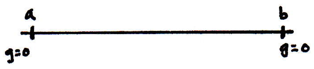
  Here's what we have, something that looks like this (we know $g$ is 0 at both $a$ and $b$):

  

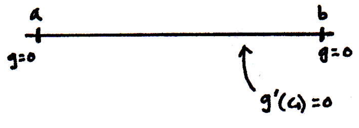
  So if we have a function that is 0 at both ends, then it either has a maximum or a minimum in between. Therefore, there's a point $c_1$ in between whose first derivative is zero. We don't know where that point is. Maybe it's here:

  

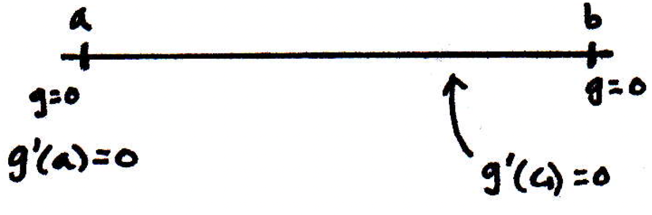
  But what do we know about $g'(a)$? It's also zero:

  

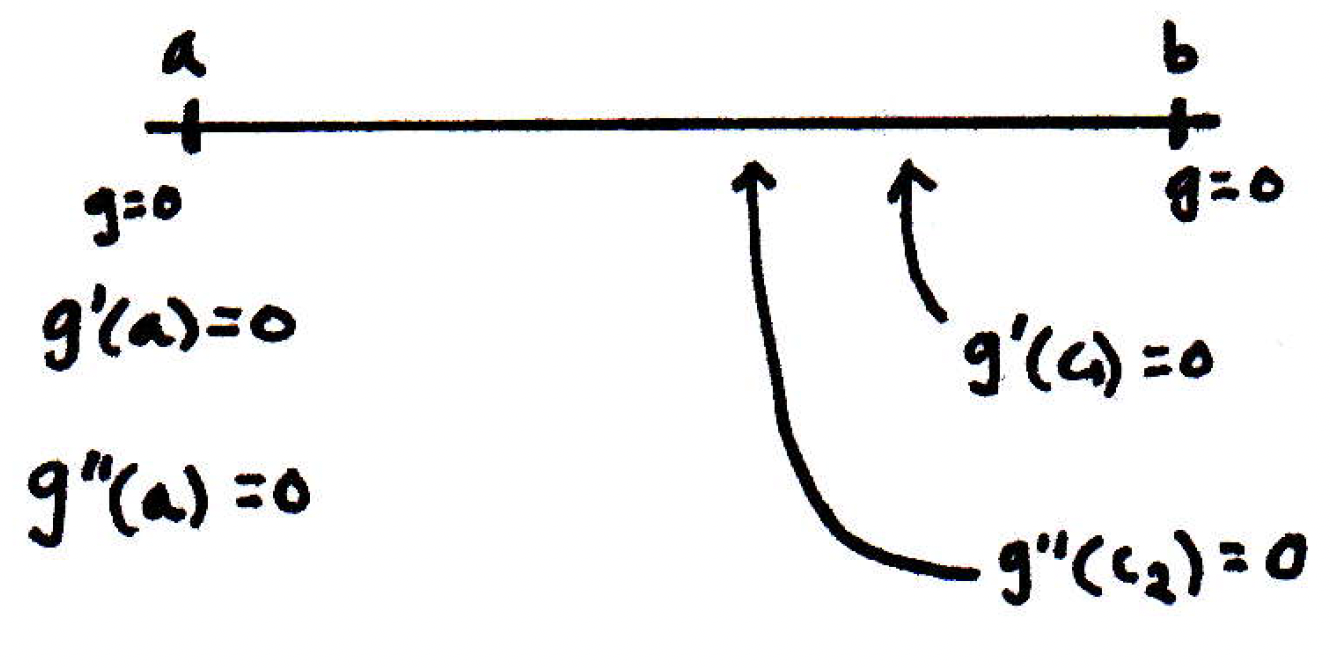
  So if we have that $g'$ is zero at both $a$ and $c_1$, then there must be a point $c_2$ between $a$ and $c_1$ where the second derivative will be zero:

  

  And we know that $g"(a)$ is also zero:

  

  We can keep going. How far can we keep going? Well, the very last step is to postulate that there is a number $c_n=c$ (this will be our chosen $c$) such that $a<c_n<c_{n-1}$, where $g^{(n-1)}(a)=0$ and $g^{(n)}(c_n)=0$:

  

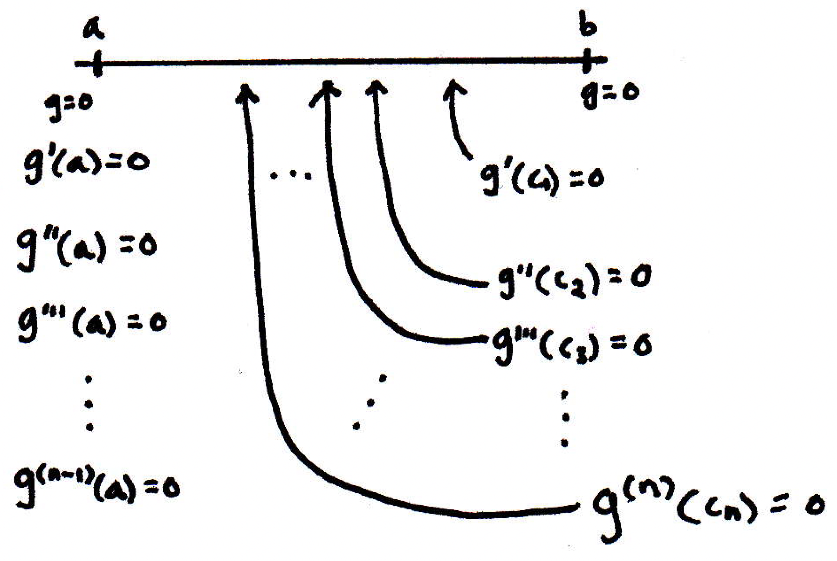
  Is that what we wanted to show? Yes, this is what we wanted to show. What is the upshot of all of this? Why does that show that $f(x)=f(x)=P_{n-1}(x)+\frac{f^{(n)}(c)}{n!}(x-a)^n$? We can plug $g^{(b)}(a)=0$ back into (1), and now (1) is true where the $b$ in (1) is playing the role of the $x$ in $f(x)=f(x)=P_{n-1}(x)+\frac{f^{(n)}(c)}{n!}(x-a)^n$. You want to know what $f(b)$ is in relation to $P_{n-1}(b)$, then that's where (1) finishes the argument. This shows that with $M=\frac{f^{(n)}(c)}{n!}$ in (1) we get the desired result.

  We should note that we used the mean value theorem several times in the argument above. We were basically bootstrapping down the derivatives through a clever choice of function.

Sequences of functions

What's special about sequences of fequences? What are they and what are they useful for?

• Preview: We've spent a great deal of time building up a lot of machinery in the first 5 chapters of Rudin that has allowed us to think about the real numbers carefully. We also built up machinery that allowed us to think about functions carefully (what it means for a function to be continuous, differentiable, etc.). What we are going to do now is point towards some ideas that will soon be encountered. One of the big ideas is that it's not just the real numbers or $\R^n$ that we're interested in. We built up all that machinery for metric spaces. What's it useful for? One of the big places where it's used is in thinking about functions living in their own metric space.

• Sequences of functions: This is actually one of the main motivations of analysis. Here's a question: We've said what it means for points to converge, but what does it mean for a sequence of functions to converge? Suppose we have a sequence

  $$f_1(x),f_2(x),f_3(x),\ldots$$

  What does it mean for a sequence of functions to converge, where we are thinking of these functions as real-valued functions? What would it really mean to say a sequence of functions converges? One way to answer this question is with the notion of pointwise convergence. Another is uniform convergence.

• Informal aside about pointwise and uniform convergence: As noted here, pointwise convergence means at every point the sequence of functions has its own speed of convergence; that is, the speed can be very fast at some points and extremely slow at others. So imagine the sequence of functions $\frac{1}{n}x^2\to0$:

  

  Think about how slow this sequence tends to zero at more and more outer points. Uniform convergence, on the other hand, means there is an overall speed of convergence, and one can check uniform convergence by considering the "infimum of speeds over all points." If it doesn't vanish, then it is uniformly convergent.

• More formal aside about pointwise and uniform convergence: It may first help to unpack the definition of limit in pointwise convergence and compare it to that of uniform convergence. The following definition for pointwise convergence is in [17]:

  Pointwise convergence (definition). Suppose $\{f_n\}$, $n=1,2,3,\ldots$, is a sequence of functions defined on a set $E$, and suppose that the sequence of numbers $\{f_n(x)\}$ converges for every $x\in E$. We can then define a function $f$ by

  $$f(x)=\lim_{n\to\infty}f_n(x)\qquad(x\in E).$$

  If this is the case, then we say that "$\{f_n\}$ converges to $f$ pointwise on $E$."

  The following definition for uniform convergence of sequences of functions is in [17]:

  Uniform convergence for sequences of functions (definition). We say that a sequence of functions $\{f_n\}$, $n=1,2,3,\ldots$, converges uniformly on $E$ to a function $f$ if for every $\epsilon>0$ there is an integer $N$ such that $n\geq N$ implies

  $$|f_n(x)-f(x)|\leq\epsilon$$

  for all $x\in E$.

  Rudin (in [17]) makes the following note about the difference between pointwise and uniform convergence:

  Difference between pointwise and uniform convergence. It is clear that every uniformly convergent sequence is pointwise convergent. Quite explicitly, the difference between the two concepts is this: If $\{f_n\}$ converges pointwise in $E$, then there exists a function $f$ such that, for every $\epsilon>0$, and for every $x\in E$, there is an integer $N$, depending on $\epsilon$ AND on $x$, such that $|f_n(x)-f(x)|\leq\epsilon$ holds if $n\geq N$; if $\{f_n\}$ converges uniformly on $E$, it is possible, for each $\epsilon>0$, to find ONE integer $N$ which will do for ALL $x\in E$.

  Hence, pointwise convergence means that for each $x$ and $\epsilon$ we can find an $N$ such that (blah blah blah). Here the $N$ is allowed to depend both on $x$ and $\epsilon$.

  In uniform convergence the requirement is strengthened. Here for each $\epsilon$ you need to be able to find an $N$ such that (blah blah blah) for all $x$ in the domain of the function. In other words, $N$ can depend on $\epsilon$ but not on $x$.

  The latter is a stronger condition, as noted in Rudin, because if you have only pointwise convergence, then it may be the case that some $\epsilon$ will require arbitrarily large $N$ for some $x$-values.

  For example, the functions $f_n(x)=\frac{x}{n}$ converges pointwise to the zero function on $\R$, but do not converge uniformly. For example, if we choose $\epsilon=1$, then the convergence condition boils down to $N>|x|$. For each $x\in\R$, we can find an $N$ easily, but there's no $N$ that works simultaneously for every $x$.

• Illustration of uniform and pointwise convergence: Consider the following picture:

  

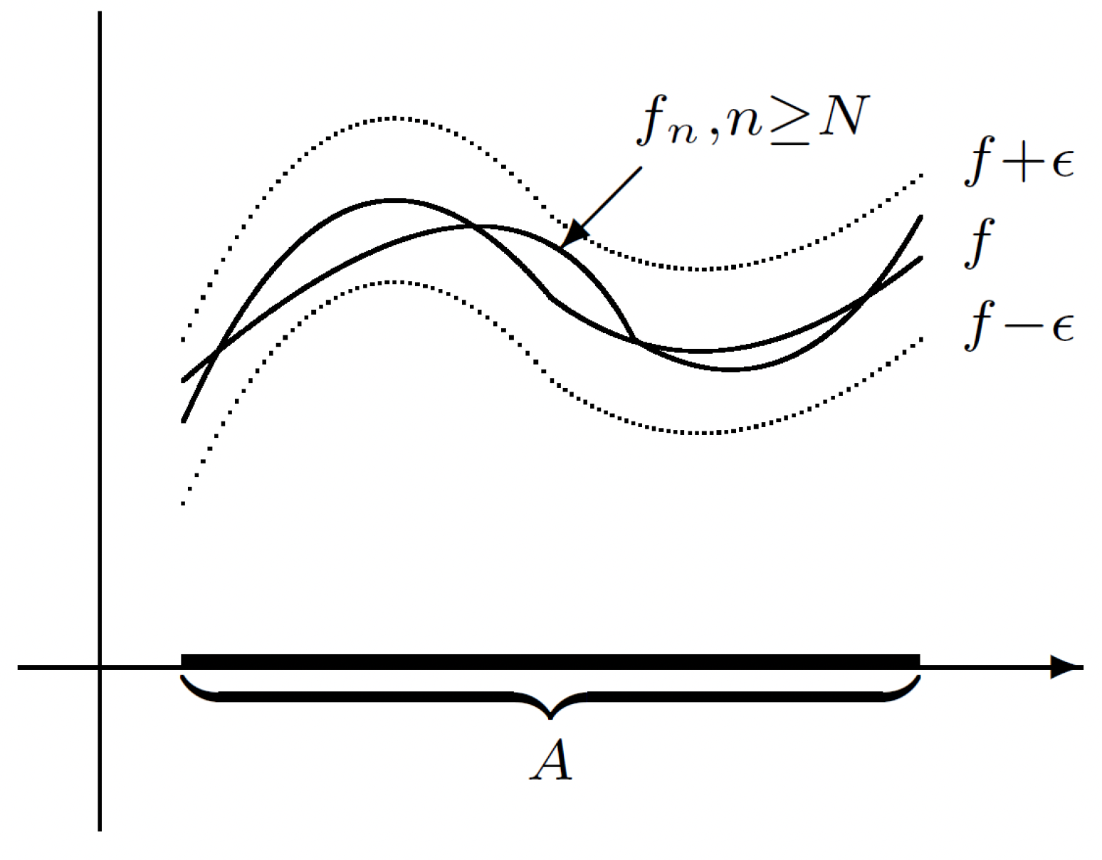
  Above we have $f_n\to f$ uniformly on $A$. Now consider the following picture:

  

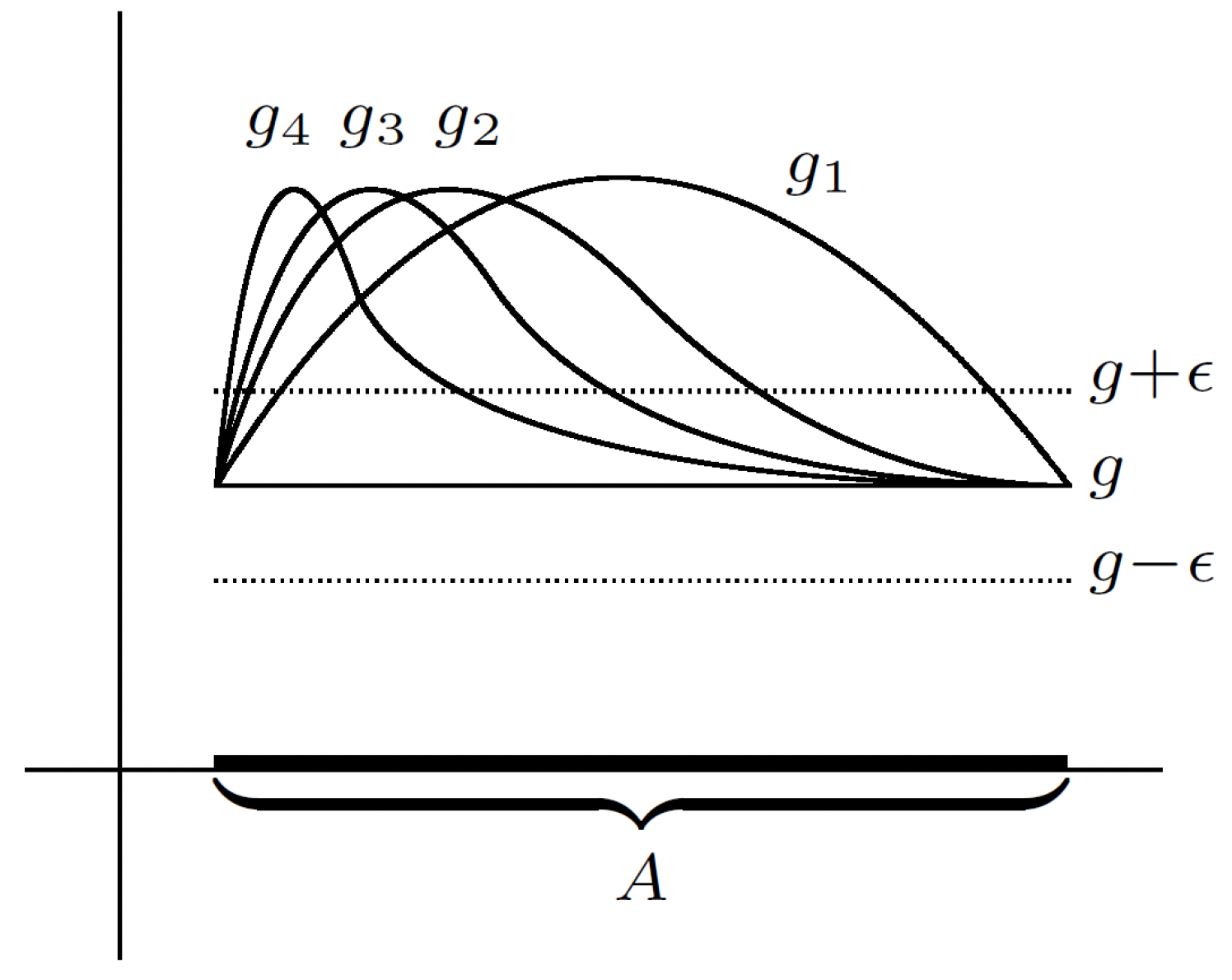
  Above we now have $g_n\to g$ pointwise but not uniformly. The difference(s) should be fairly clear.

• Returning to Su lecture (concerning pointwise convergence): Fix $x$, and ask yourself whether or not $\{f_n(x)\}$ evaluated at a particular point converges? If it does, then we say that $\{f_n\}$ converges pointwise, and we write the so-called pointwise limit as $f(x)=\lim_{n\to\infty}f(x)$. (Note this is a sequence of numbers since we are evaluating the functions at a point.)

• Example of pointwise convergent function: Consider the following sequence of functions: $f_n(x)=\frac{x}{n}$. What is the pointwise limit of this sequence? Does this converge pointwise? Yes. To the zero function. So we can write $f_n(x)=\frac{x}{n}\stackrel{\text{pointwise}}{\longrightarrow} f(x)=0$.

• Another example: Consider the sequence $f_n(x)=x^n$ on $[0,1]$. Does this converge pointwise? We see that $f_1(x)=x$, $f_2(x)=x^2$, $f_3(x)=x^3$, etc. Does this converge pointwise? We'd have something that looks like the following for the first few functions:

  

  So the $f_n$ stays at 1 for $x=1$ and goes to $0$ everywhere else on $[0,1]$ only. Interesting. So

  $$f_n(x)=x^n\stackrel{\text{pointwise}}{\longrightarrow} f(x)= \begin{cases} 1 & \text{at}\ x=1,\\ 0 & \text{otherwise}. \end{cases}$$

• Another example: Consider the following function:

  

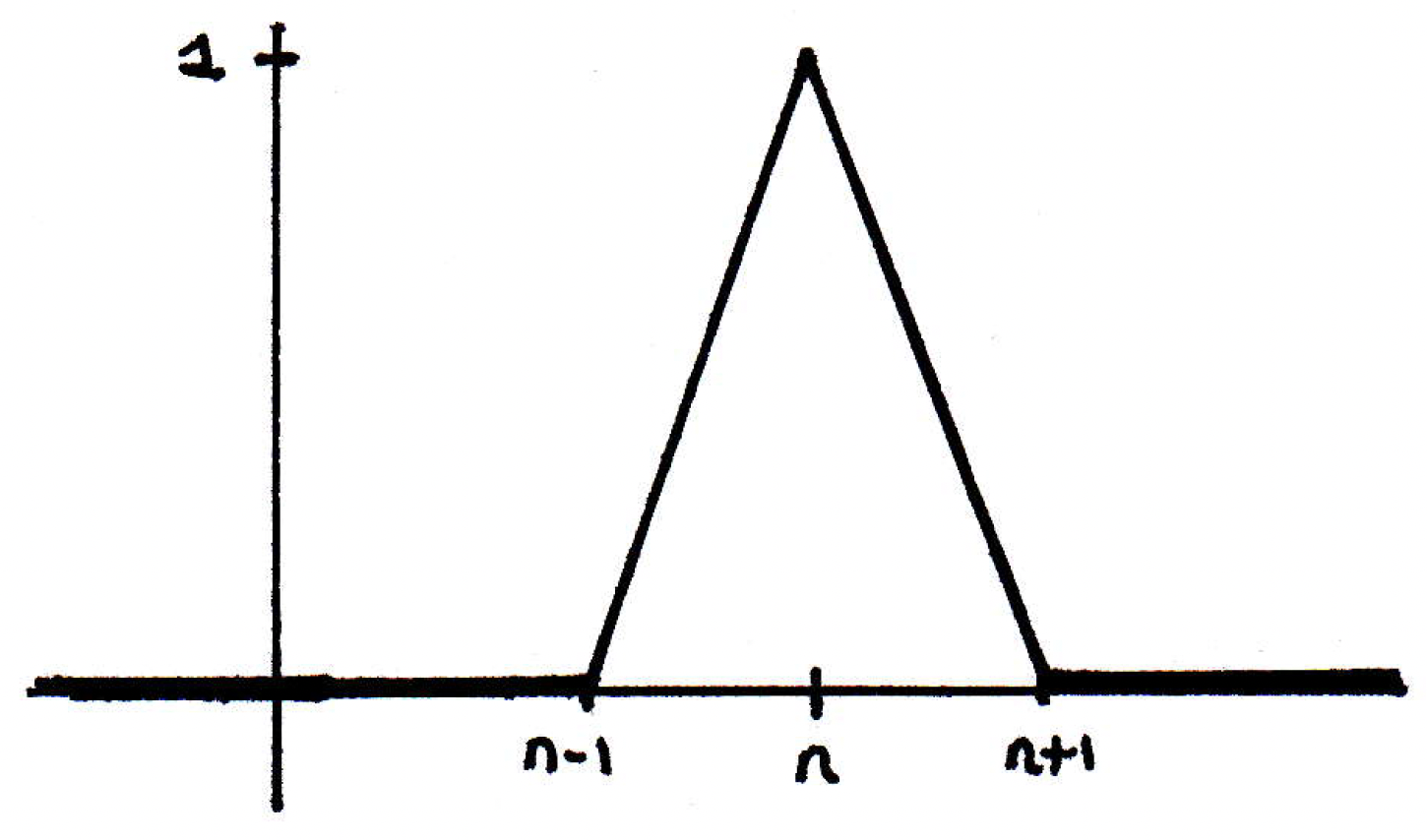
  So this function has a spike at $x=n$, and it lives between the next two integers, $n-1$ and $n+1$. So $f_1(x)$ would have a spike at $x=1$, $f_2(x)$ would have a spike at $x=2$, etc. We would have $f_n\stackrel{\text{pointwise}}{\longrightarrow}f(x)=0$. Fascinating. This is an interesting notion of convergence. Is it the best notion is it the right notion?

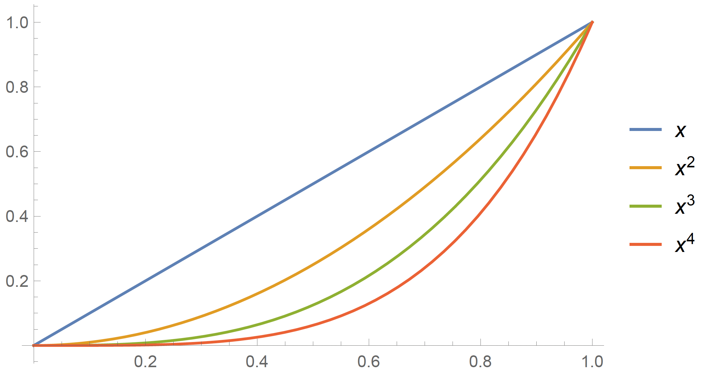
• Another example: How about $f_n(x)=\frac{1}{n}\sin(n^2 x)$? We'd have something that looked like the following for the first few terms of the sequence:

  

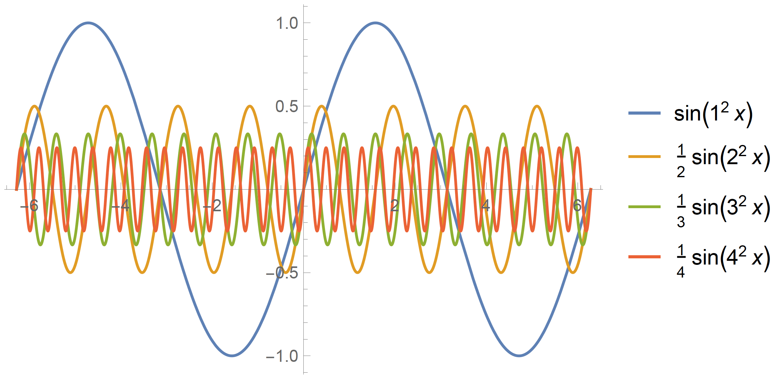
  What does this converge to, if anything? It turns out that

  $$f_n(x)=\frac{1}{n}\sin(n^2 x)\stackrel{\text{pointwise}}{\longrightarrow} f(x)=0.$$

  Don't be fooled! Not all sequences of functions converge to 0.

• Reflection: What can we learn from the examples above? They exhibit some very interesting behavior. Here's the kind of question we've been dealing with when you have sequences: What properties are preserved by the limiting operation for functions? What properties are preserved by pointwise limits? For example, is it true that the pointwise limit of a continuous function is continuous? No. Why? We saw this debunked with the example where we considered $f_n(x)=x^n$ on $[0,1]$.

  What about derivatives? If we take the derivative of a limit is it the limit of the derivatives? And a very good example of this is in physics where you have an infinite sum, and you're asked to take the derivative of an infinite sum and you do it term by term. Isn't an infinite sum like a limit? A limit of partial sums? So are derivatives preserved by limits? No. In fact, with $f_n(x)=\frac{1}{n}\sin(n^2 x)$ we see the derivatives are starting to behave very wildly. And the derivative of the limit is 0. So this is not true in general.

  What about integrals? So think about areas. Are they preserved by pointwise limits? No. In fact, the example with the spike is a counterexample to this idea.

  Right now things do not look very nice. Indeed, some of the most desirable properties, namely continuity, differentiability, and integrability, are not preserved with pointwise limits. So we need something stronger to help us. Maybe it will help some of our issues here. Maybe not all of them but some. (Much of this is discussed in the next analysis course.) Let's look at $||f||=\sup_{x\in E}|f(x)|$. So the $\sup$ of the spike function would be what? It would be 1. What about the $\sup$ of $f_n(x)=\frac{x}{n}$ over the entire domain? Yeah, infinite. We don't like that. If we restricted the domain, then the function would have a supremum. Let's make a definition of something we can get at that may be of some use.

• Uniform convergence: We should first diligently note that uniform convergence and uniform continuity are completely different concepts. But the word "uniform" is supposed to make us think of what? Everybody's wearing the same uniform. So what is behaving uniformly here?

  We write $f_n\stackrel{u}{\to} f$ on $E$ (i.e., $f_n$ converges uniformly to $f$ on $E$) if for all $\epsilon>0$ there exists $N$ such that $n\geq N$ implies $||f_n-f||<\epsilon$.

  How is this like or unlike the notion of convergence that we have previously encountered? What's uniform about the idea? What's different from this definition compared to that of pointwise limits, which also asks you to take a limit of a sequence? The idea here, because we are looking at the supremum of a difference, and we are demanding that that be less than $\epsilon$, we're going to have "ribbon convergence." You can drawn an $\epsilon$-ribbon about $f$ and $f_n$ eventually stays within the ribbon. What's uniform is that the same $N$ works for every $x$.

• Dealing with uniform convergence: Would we say $f_n(x)=\frac{x}{n}$ is uniformly continuous? No, these function are not all living in the $\epsilon$-ribbon eventually. In fact, every single function eventually leaves the ribbon. What about the sequence function $f_n(x)=x^n$ for $x\in[0,1]$? Does this converge uniformly? No, you'll still have problems no matter how far you go, where the functions do not lie completely inside the ribbon. What about the spiky function? Also not uniformly continuous. (Choose $0<\epsilon<1$.) What about the sequence $f_n(x)=\frac{1}{n}\sin(n^2 x)$? This does converge uniformly. So not all of our problems will be solved with ribbon or uniform convergence. But some of them will be hopefully.

• Note about metric spaces: What we've done is placed all of the functions in their own metric space, and by defining $||f||=\sup_{x\in E}|f(x)|$ to be the distance on this space, we have our distance function (i.e., the supremum distance) for our metric space. The concept of convergence just discussed is the "usual convergence" in the metric space $C_b(E)$, where $C_b(E)$ represents the continuous bounded functions on $E$. So really we're just letting $d(f,g)=||f-g||$. So what's so great about this metric space? So we are thinking about every function as a point in its own space:

  

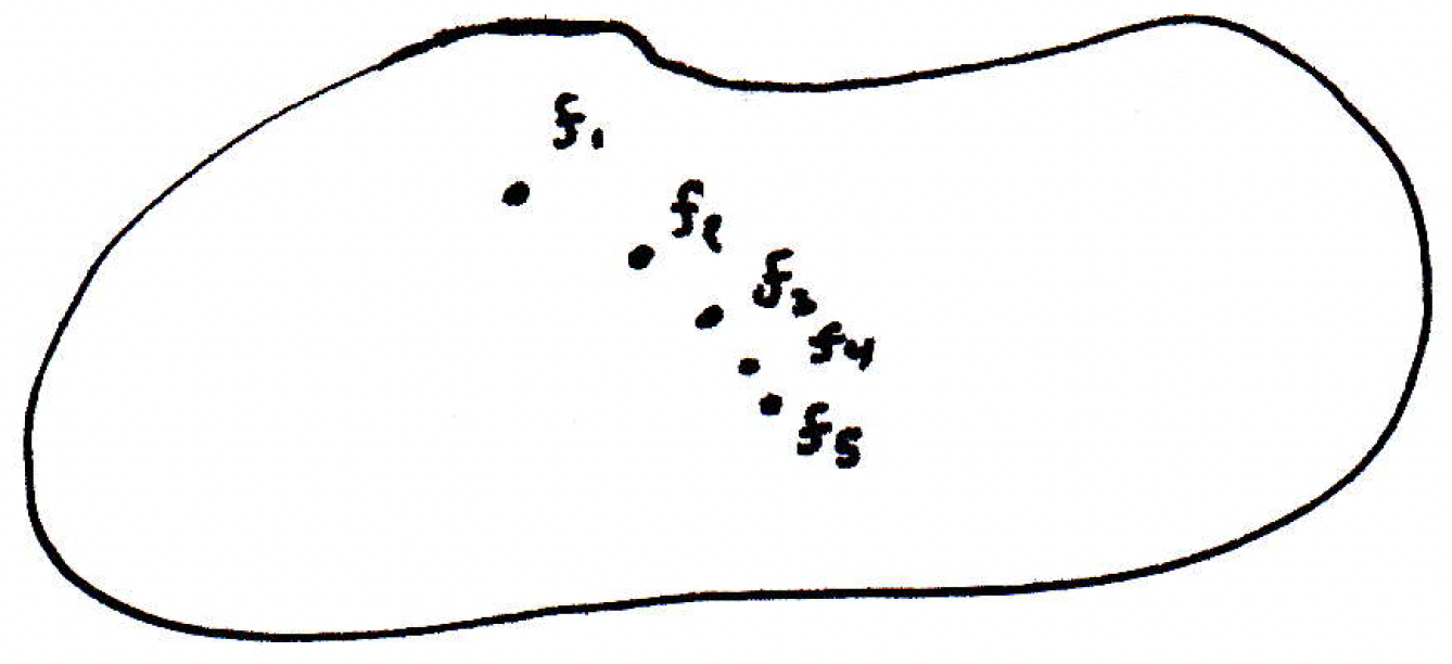
  So uniform convergence is just like regular convergence in this space. So if we have a sequence of functions, must the sequence converge? Not necessarily. Well, what would we like to know about the space above in order for a sequence to converge? Is it complete? Here's a big fact from the next course in analysis: The space of functions $C_b(E)$ is complete. So, in fact, we have a Cauchy criterion. This will allow us to say, without knowing what the limit is, whether or not a limit exists. Let's just see if the functions form a Cauchy sequence. That's a theorem.

• Theorem about convergence of sequences of functions: We have $f_n\stackrel{u}{\to} f$ if and only if for every $\epsilon>0$ there exists $N$ such that for all $n,m\geq N$ and for all $x\in E$, we have that $|f_n(x)-f_m(x)|<\epsilon$. (Note the replacement of double norm signs. We're saying the same thing.) This is the Cauchy criterion for uniform convergence.

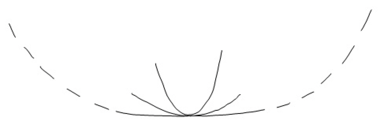
• Example (Koch snowflake): Consider $f_n\colon[0,1]\to\R^2$, where $f_1$, $f_2$, $f_3$, and $f_4$ looks as follows (top left to bottom right, respectively):

  

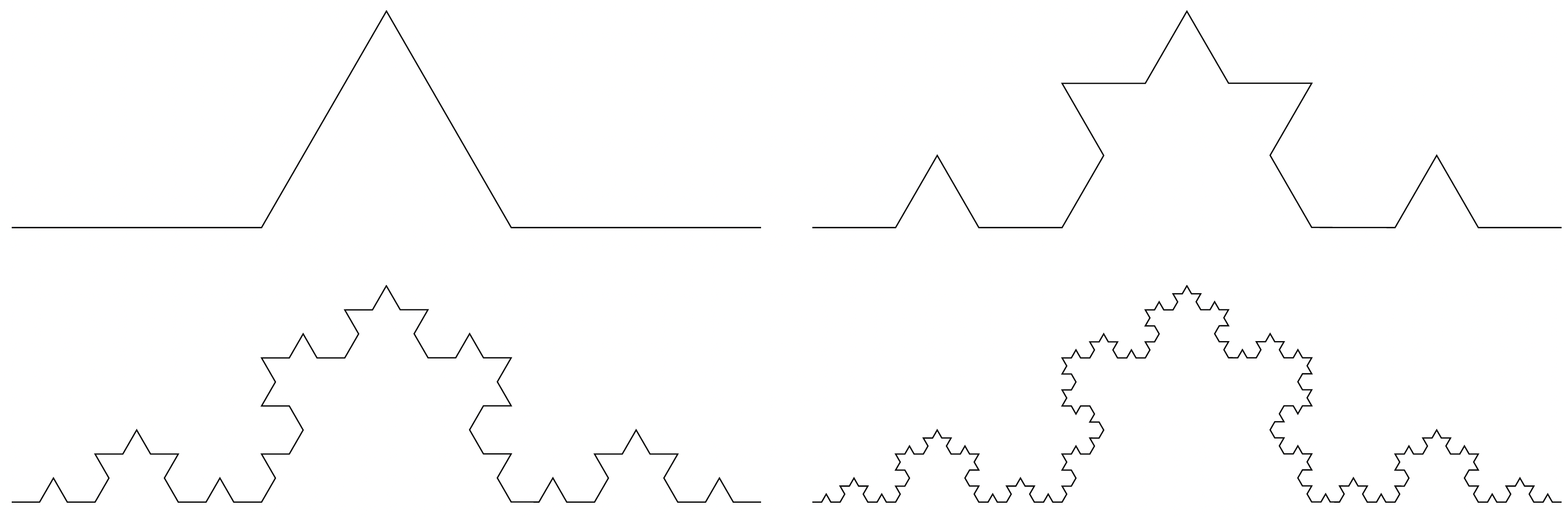
  This is the construction of the Koch snowflake. It's a fractal-like construction. But what do people say the snowflake is? Well, it's the one you get by taking the limit of these functions. But how do we know the limit exists? How do we know the sequence is Cauchy? Successive distances are smaller and smaller. In fact, past some point, for a fixed $x$, all of the terms $|f_n(x)-f_m(x)|$ will be close (or simply $|f_n(x)-f_m(x)|<\epsilon$). Essentially, by construction, we see that $f_n$ is Cauchy. (We could be very careful in defining the function to ensure proper conditions are met.) So it converges. So we know the fractal limit exists. Of course, now the question is what is the limit? Here's a theorem.

• Theorem: If $f_n\stackrel{u}{\to} f$, with $f_n$ all continuous, then $f$ is continuous.

  Is this true in general for pointwise convergence? No. But it is true for uniform convergence. The ribbon kind of convergence helps us. It means that the limit is, in fact, continuous. What does that mean for the snowflake curve? The limiting function is continuous because of this theorem. So the Kock snowflake is continuous. Let's prove this.

• Theorem proof: Here's the idea: Consider the operative bound

  $$|f(x)-f(y)|\leq|f(x)-f_n(x)|+|f_n(x)-f_n(y)|+|f_n(y)+f(y)|,$$

  where we let $\alpha=|f(x)-f_n(x)|$, $\beta=|f_n(x)-f_n(y)|$, and $\gamma=|f_n(y)+f(y)|$ for ease of reference. So our operative bound becomes

  $$|f(x)-f(y)|\leq|f(x)-f_n(x)|+|f_n(x)-f_n(y)|+|f_n(y)+f(y)|=\alpha+\beta+\gamma.$$

  Fix $x$. For all $\epsilon>0$, choose $f_n$ so $||f_n-f||<\frac{\epsilon}{3}$. So $\alpha,\gamma<\frac{\epsilon}{3}$. What's the second choice? Then $f_n$ is continuous. Thus, there exists $\delta>0$ such that if $|x-y|<\delta$ then $\beta<\frac{\epsilon}{3}$. So for every $\epsilon>0$, we found a $\delta$ such that

  $$|f(x)-f(y)|<\frac{\epsilon}{3}+\frac{\epsilon}{3}+\frac{\epsilon}{3}=\epsilon,$$

  as desired. We will have one last application.

• Theorem: There exists a function $f\colon[0,1]\to[0,1]^2$ that is space-filling. That is, we claim there is a function from the interval $[0,1]$ into the "box" $[0,1]^2$ that completely fills out the entire box. It hits every point. How is that possible? We have a compact interval $[0,1]$, and we're saying it will fill out the whole thing? Well, it's actually quite easy to show using the above theorem because we'll just construct the space-filling curve as a limit of a sequence of functions that is uniformly convergent. And we'll do this by making it Cauchy.

  The basic idea is to start with the box, divide it up into thirds, and then wind your way through:

  

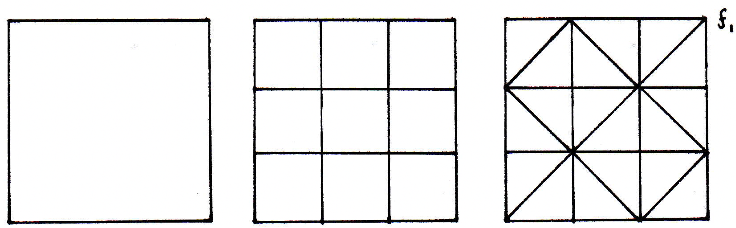
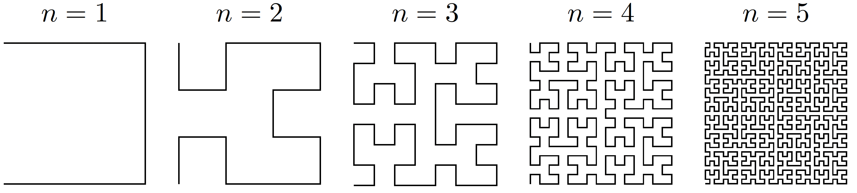
  There are many ways to do this. The above is just an illustration of how to get started with one approach. Given the $f_1$ we constructed, what will $f_2$ look like? The basic idea is to now cut each of the nine little squares into tic-tac-toe grids themselves (so now you would have 81 little squares in total) and replace each of those lines with the construction of the far right figure above. And keep doing this. Doing so will fill the box. Why is this converging uniformly? Well, you can convince yourself that everything stays within a little box (all the images of particular points for a fixed time stay within a box) past some point so it converges uniformly. It converges in a Cauchy sense. So it must converge to a limit, and you can show that every point in the box is actually the pointwise limit of some point. So it fills out all of the space. So there exists a space-filling curve. Another space-filling curve is the Hilbert curve which looks like the following for $f_1$, $f_2$, $f_3$, $f_4$, $f_5$:

  

  We can actually construct these space-filling curves in $\R^3$ if we like:

  

  We could actually construct these space-filling curves in $\R^n$ as well.