20 - Functions - limits and continuity

Functions in arbitrary metric spaces

What is the deal with functions in arbitrary metric spaces? What is a function? What does it mean for a function to have a limit? And what does it mean for a function to be continuous?

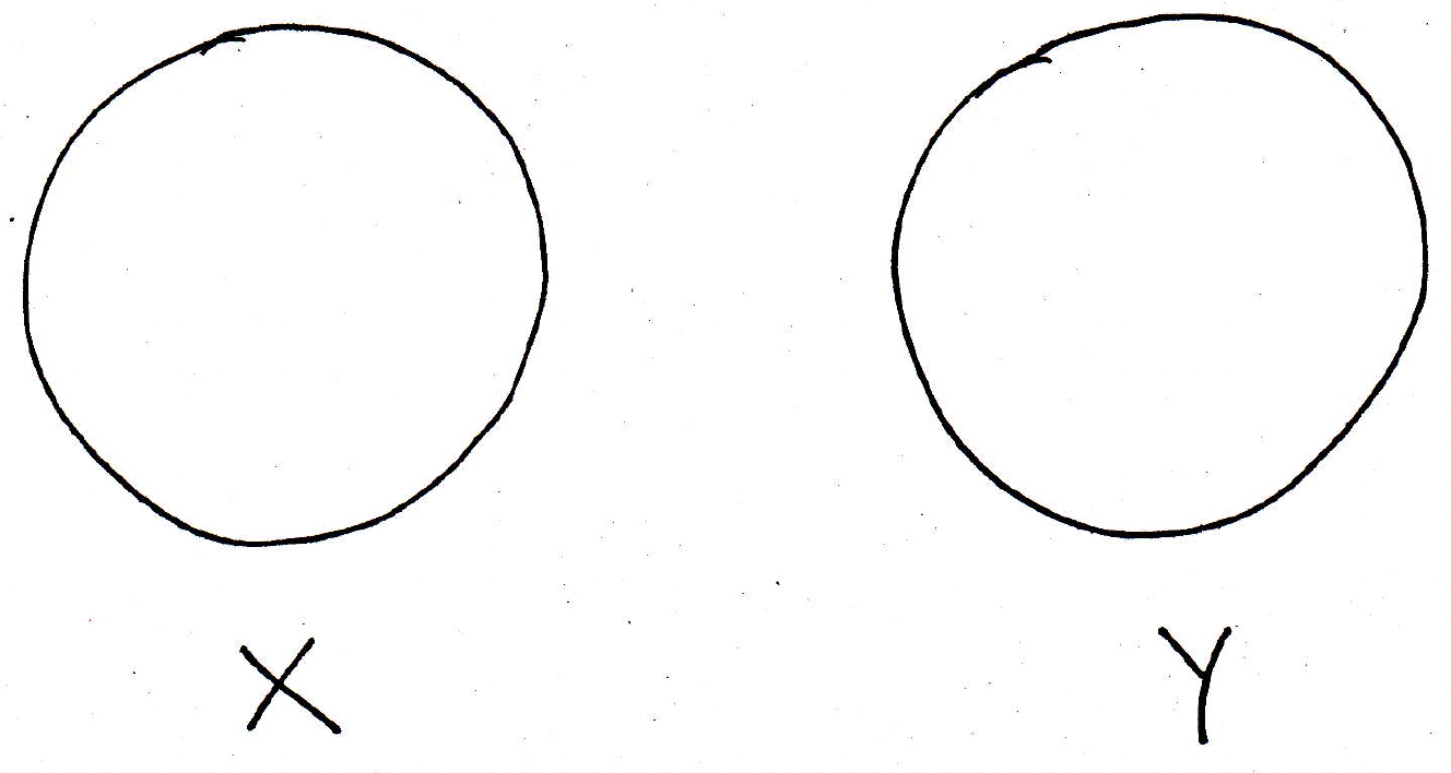
• Functions: Throughout the lecture, we will imagine we are dealing with two metric spaces, $X$ and $Y$. So let $X$ and $Y$ be metric spaces. So each of them has some metric or some notion of distance on them. We might think of $X$ and $Y$ in the following way:

  

  A function is going to be an assignment, and we actually defined this at the very beginning of the class. The function will be an assignment of a point in $X$ to a unique point in $Y$. We may even have a whole line of things being mapped to another line in $Y$:

  

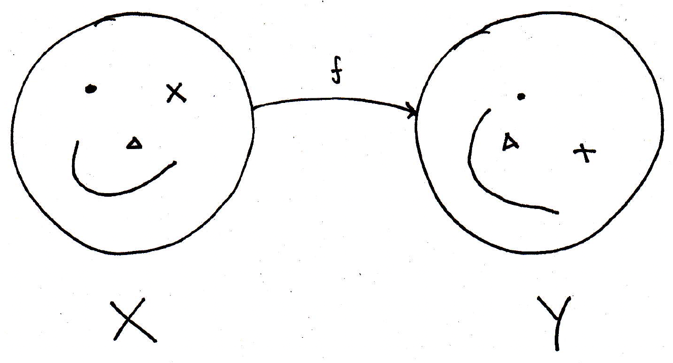
  There are, of course, many ways to think of functions. Separating a function into its domain and codomain is a very mathematical way of looking at functions, but you've also seen throughout your education that you can visualize functions as graphs. So in the picture above, we have a mapping, but we could also think about $f$ as a graph. Of course, if we are trying to look at $f$ as a graph, then we would try to put these things on the same diagram where we place $X$ and $Y$ as follows:

  

  With the mapping representation of the faces, the domain and codomain were both 2-dimensional, and so on the $X$-axis you would have two dimensions and on the $Y$ axis you would have two dimensions. It is fairly easy to see that the graph quickly becomes intractable when the dimensions get bigger than 3 because the graph of a function from 2 dimensions to 2 dimensions will be 4-dimensional. This is why often it's a better picture to think about the oval mapping of elements from one set to another set than the strict graph interpretation.

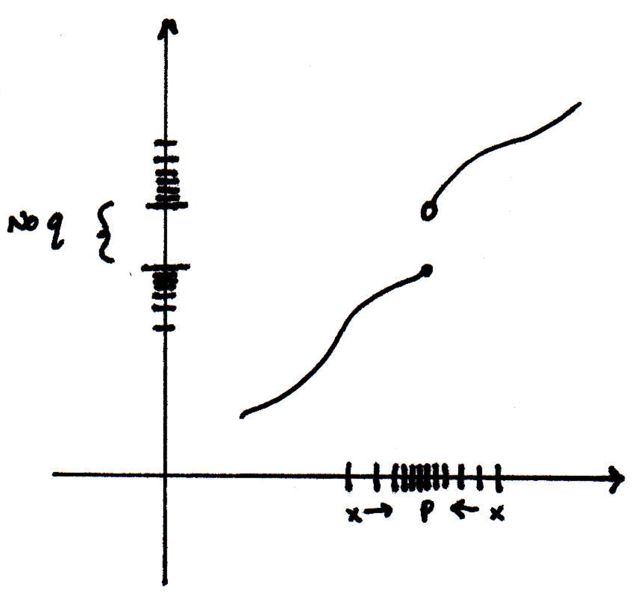
• Limits: What does it mean to talk about the limit of a function? That's the question we want to grapple with. We've already talked about what it means to take limits of sequences. We know what this means: $\lim_{n\to\infty} x_n=x$. It means that for every $\epsilon>0$ there is an integer $N$ such that for all $n\geq N$ we have $d(x_n,x)<\epsilon$ or $|x_n-x|<\epsilon$ using the usual metric, but what we want to grapple with is the following question: Does it make any sense whatsoever to talk about the limit of a function:

  $$\lim_{x\to p}f(x)=q.$$

  What does this mean? Can we make sense of this? So let's just look at some examples.

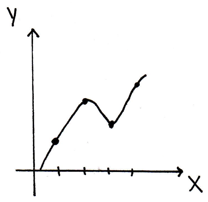
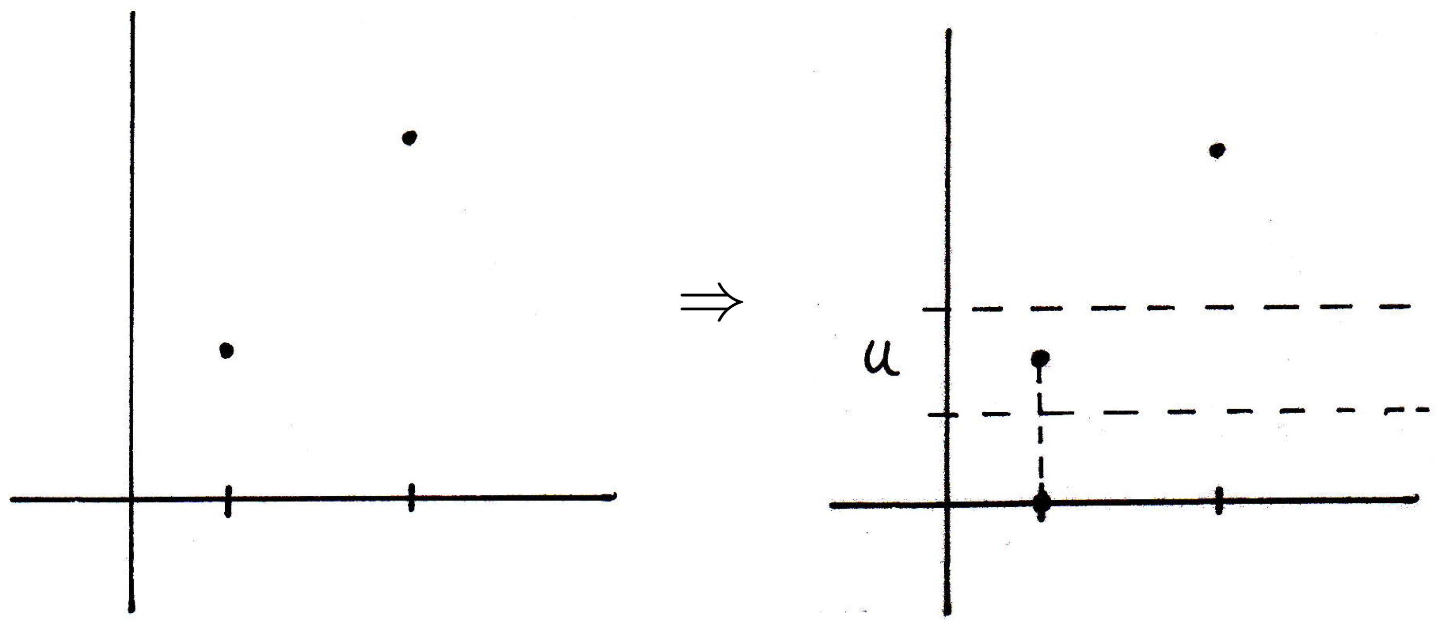
• Example 1: So maybe we draw the graph of a particular function. It might look something like this:

  

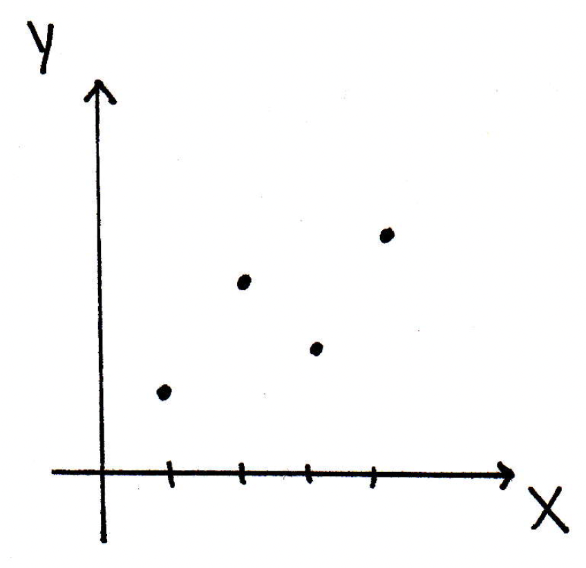
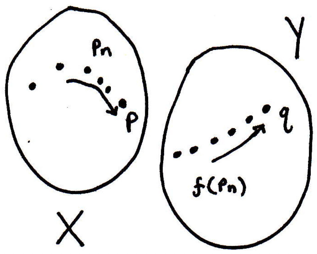
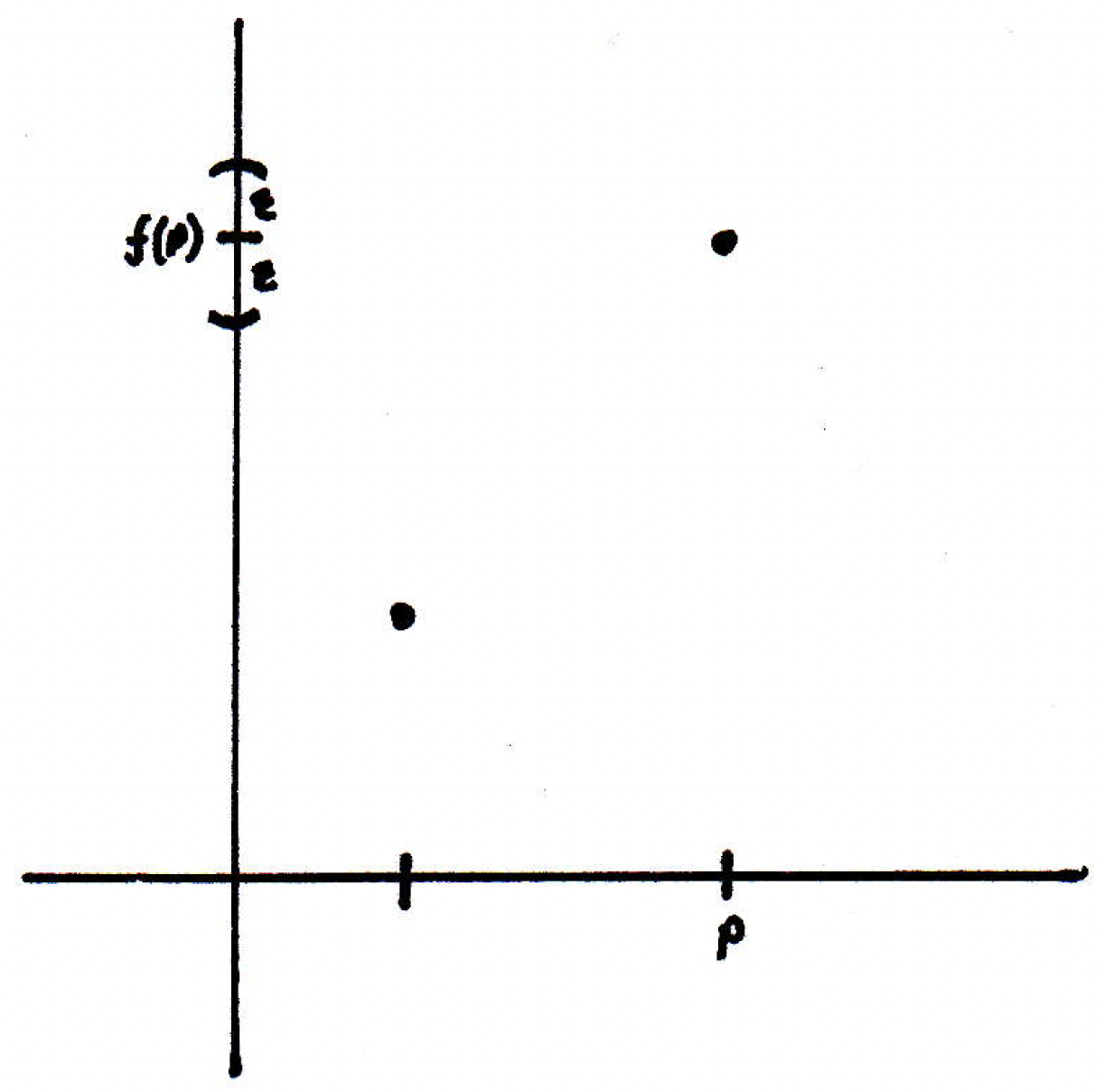
  So what we've depicted is four points in the domain $X$ that go to some four points in the range, and we've just graphed them here. This is at least part of a function. Maybe we haven't defined the whole function, but does it make any sense to say that $f(x)$ goes to some $q$ as $x$ goes to some $p$? Here, of course, we only have 4 points, but you could imagine we have a whole interval of points in the domain and we know where they go in the codomain. So maybe the picture would look like the following if we showed all of the points:

  

  And then we could begin to ask if a bunch of points down on the $X$-axis converge to $p$, then what does that mean? Can we say that their images converge to some $q$ in $Y$? That's kind of the question we are asking:

  

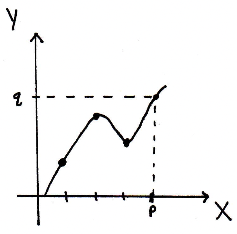
• Example 2: Maybe our graph of a function looks something like this:

  

  So we have a point $p$ and a bunch of $x$'s going to $p$, and now the question is can we talk about the limit of the $f(x)$'s. Are these points doing something? That's the question. How do we make sense of this?

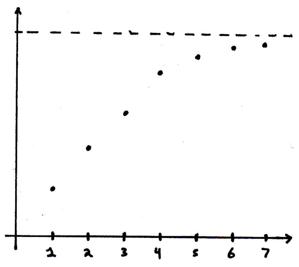
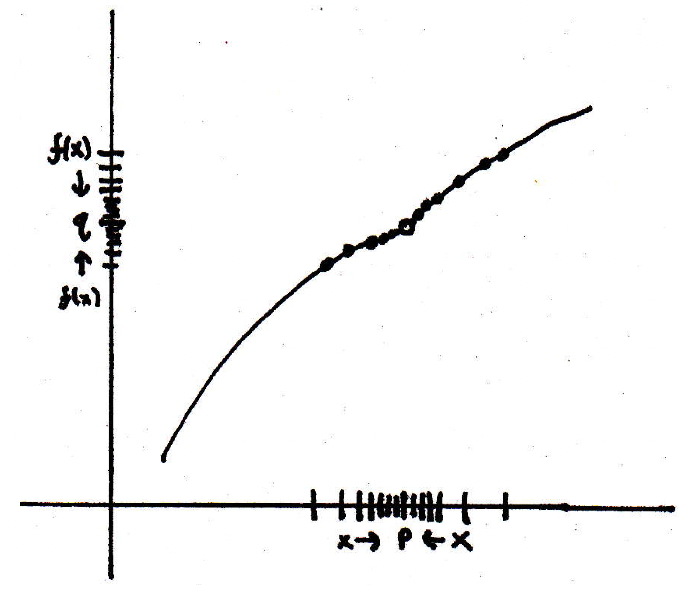
• Example 3: What we should first notice is that the statement about the limit of a sequence is actually a statement about a function since a sequence is a function is it not? How is a sequence a function? It takes in an index and spits out a number. So that's a function that looks something like this, where it's defined only on the integer points, and if it was converging to some kind of limit, then really what we are saying is that, as we go further and further out, the graphed points approach a limiting value (indicated by the dashed line below):

  

  What's different about $\lim_{x\to p}f(x)=q$ as opposed to $\lim_{n\to\infty} x_n=x$ is that we are allowing ourselves to look at points that do not go off to infinity but maybe get closer and closer to $p$, and we are asking ourselves something about what $f(x)$ is doing. This should hopefully motivate our definition of limits. Let's see if we can make a precise definition below.

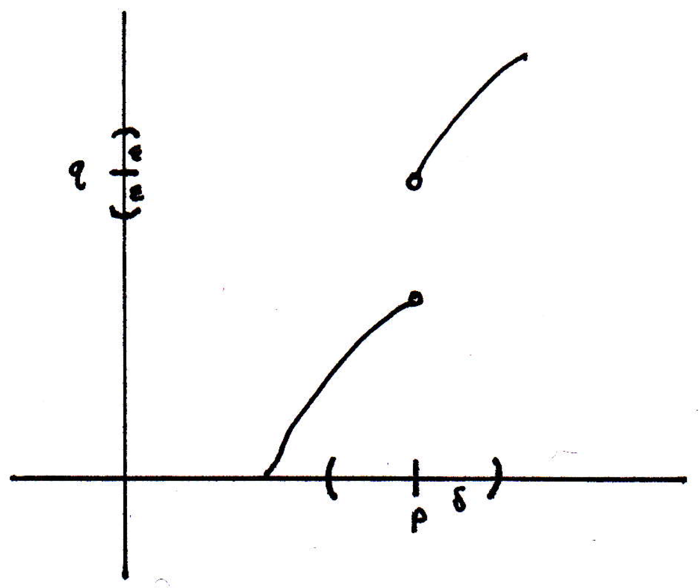
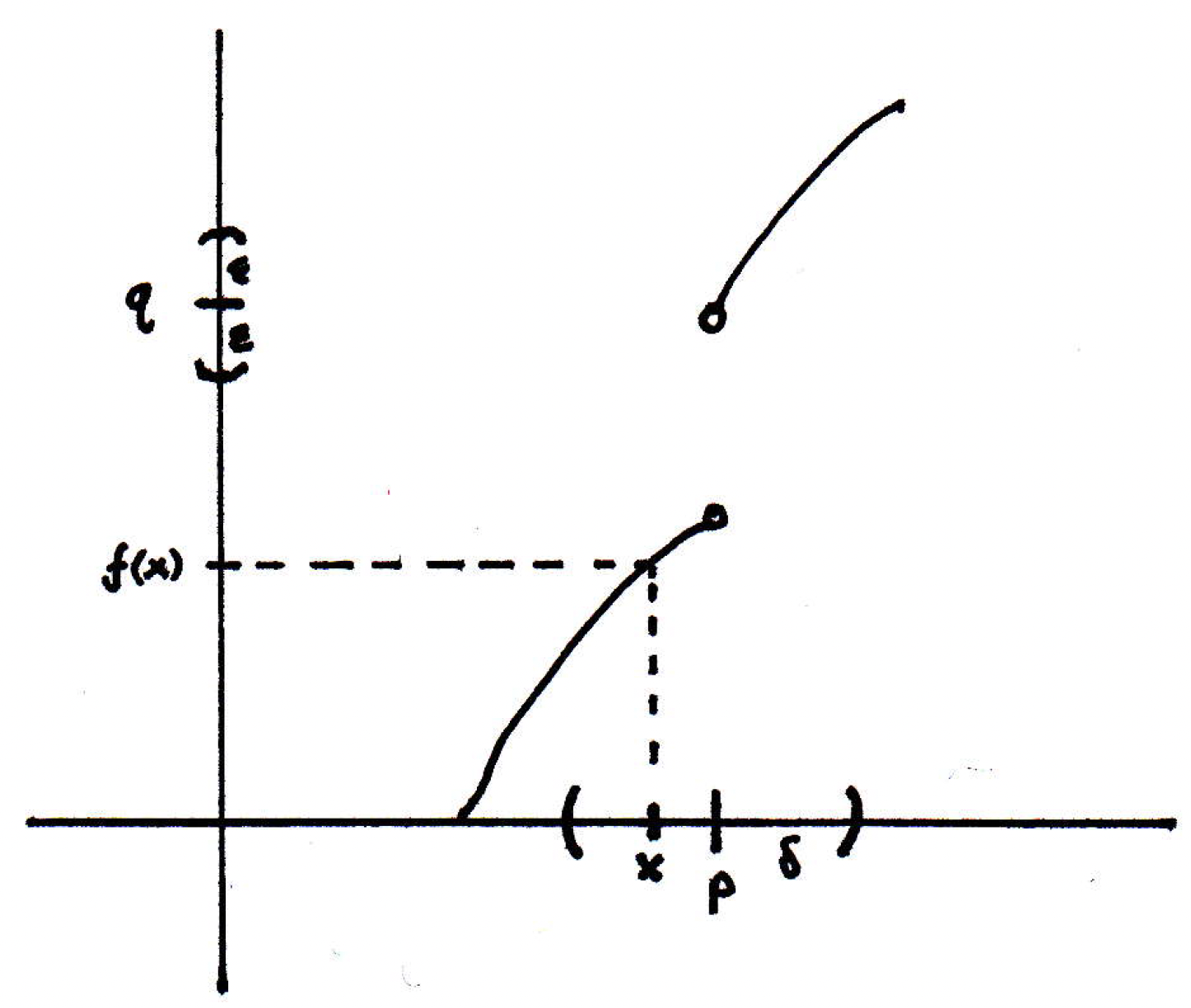
• Limit (definition from Su based on Rudin): Let $X$ and $Y$ be metric spaces where $E\subset X$, and let $p$ be a limit point of $E$. Let $f\colon E\to Y$. So we have a space $X$ and a space $Y$, and we're only interested, perhaps, in some subset $E$ of the domain $X$, and a function from this subset to $Y$ perhaps:

  

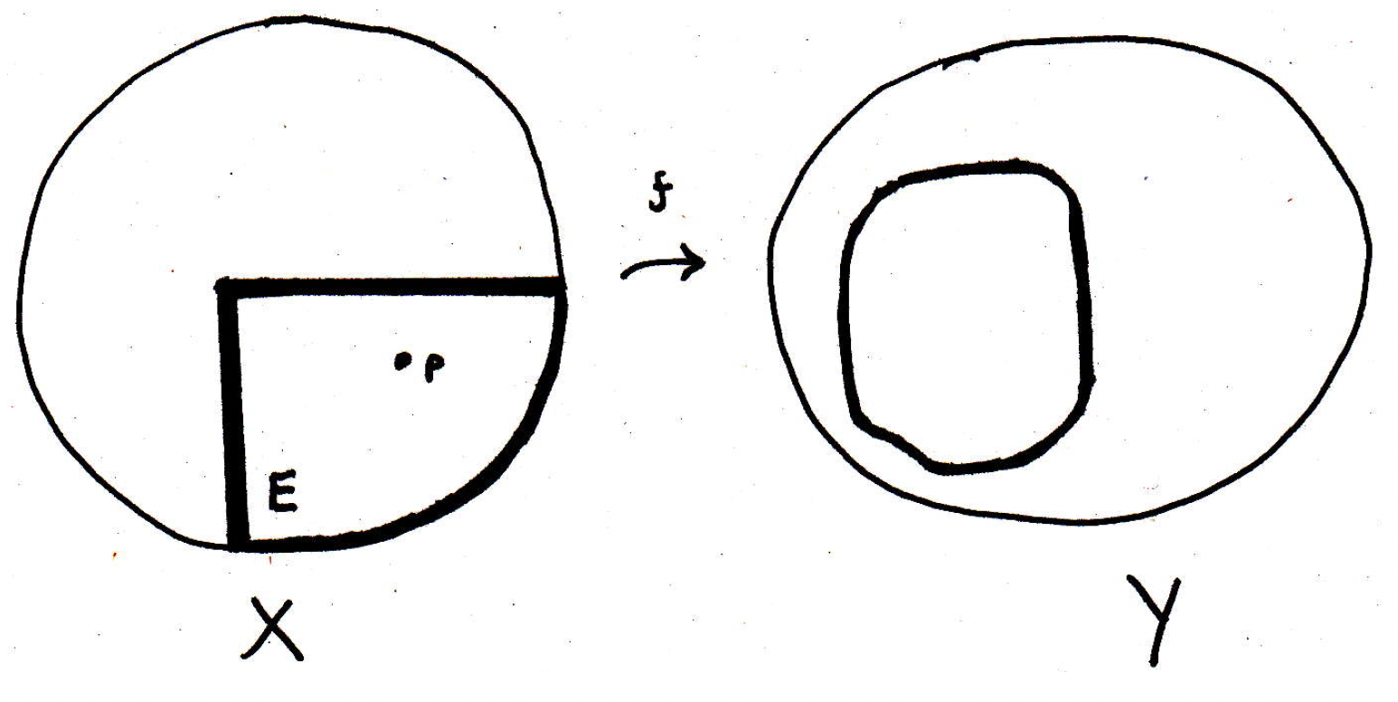
  We have our set $E$ above, and we are going to be picking $p$, a point that is a limit point of $E$ so it should be possible to converge or get closer and closer to $p$ in $E$. And now we're asking does a particular limit exists? What does that mean intuitively from the picture above?

  We'll say our function has a limit, and we'll call it $q$, if whenever we have a bunch of points getting closer and closer to $p$ then their images are getting closer and closer to $q$:

  

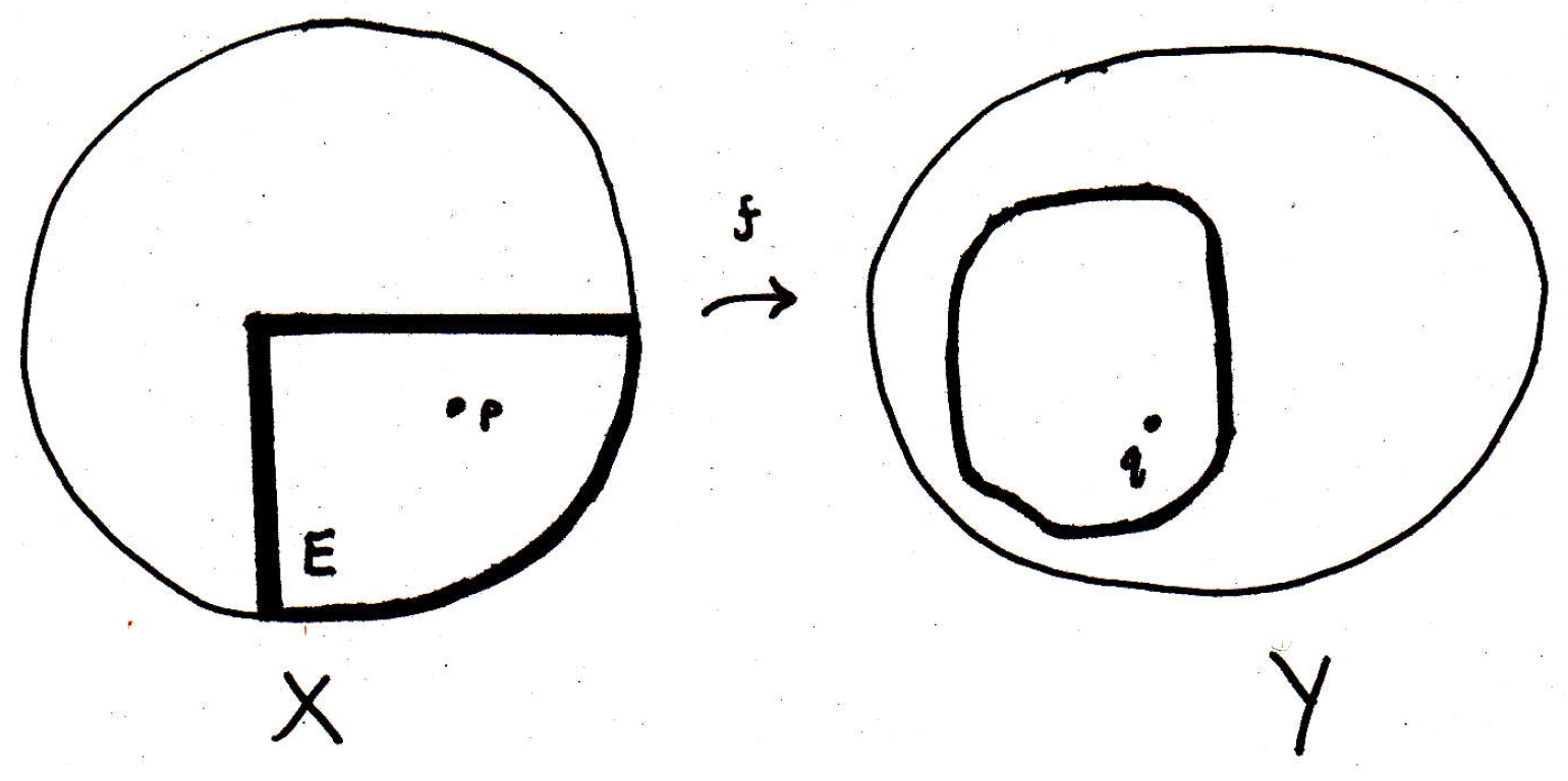
  The way this potential definition has been described has largely been done almost as a sequence of points. That's one way to describe this limit, but let's first do this in terms of distances. We will develop a criterion that looks something like the convergence criterion for sequences. As a side note, we should observe that $p$ does not have to be in $E$ (it could be on the boundary), and there's no relationship between $p$ and $q$ necessarily other than the fact that as points get closer and closer to $p$, the images of these points must be getting closer and closer to $q$, but it need not be the case that $q$ is the image of $p$.

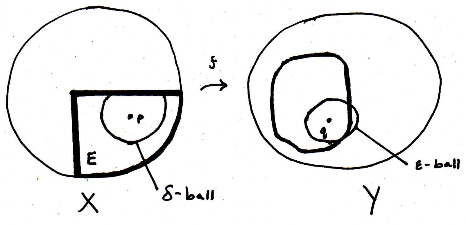
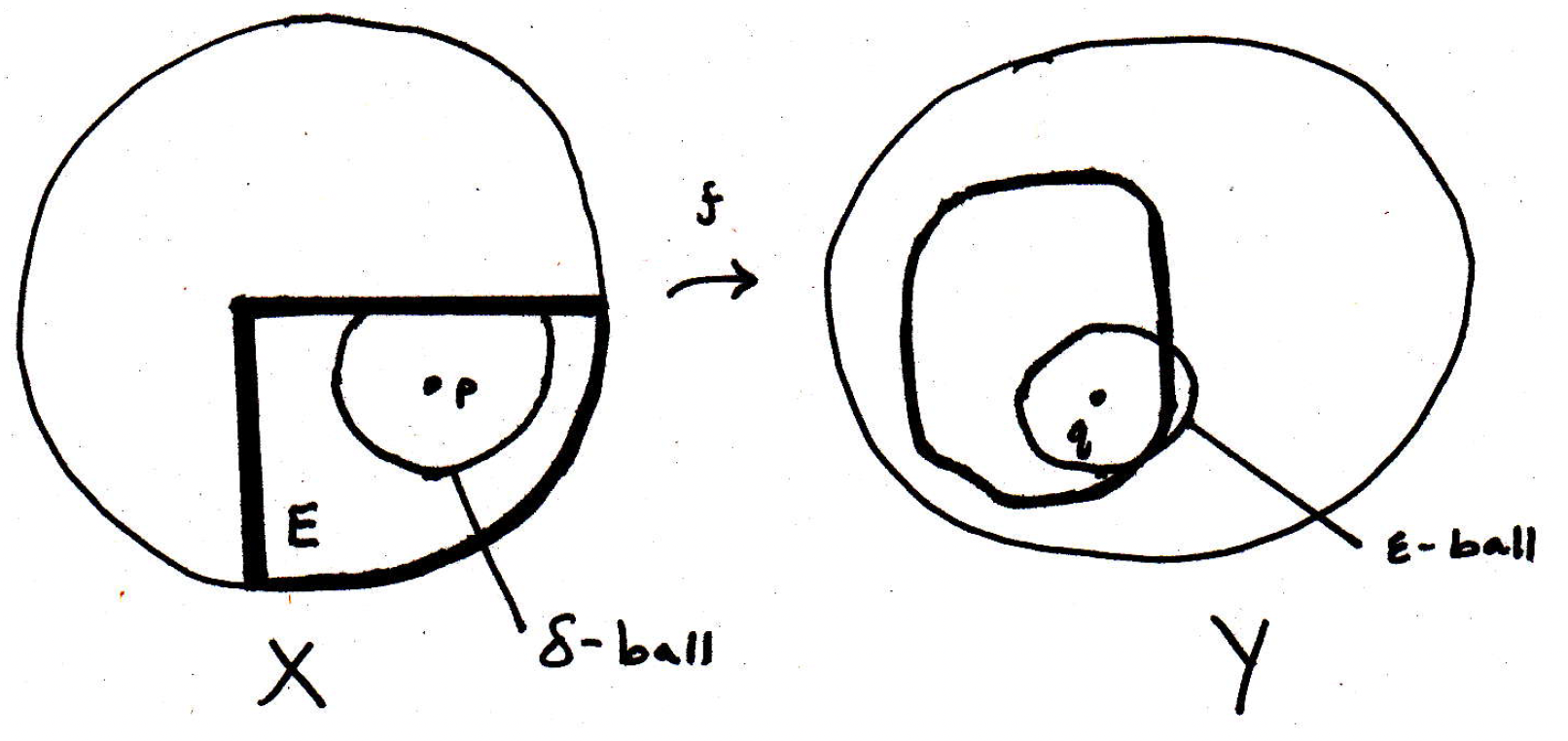
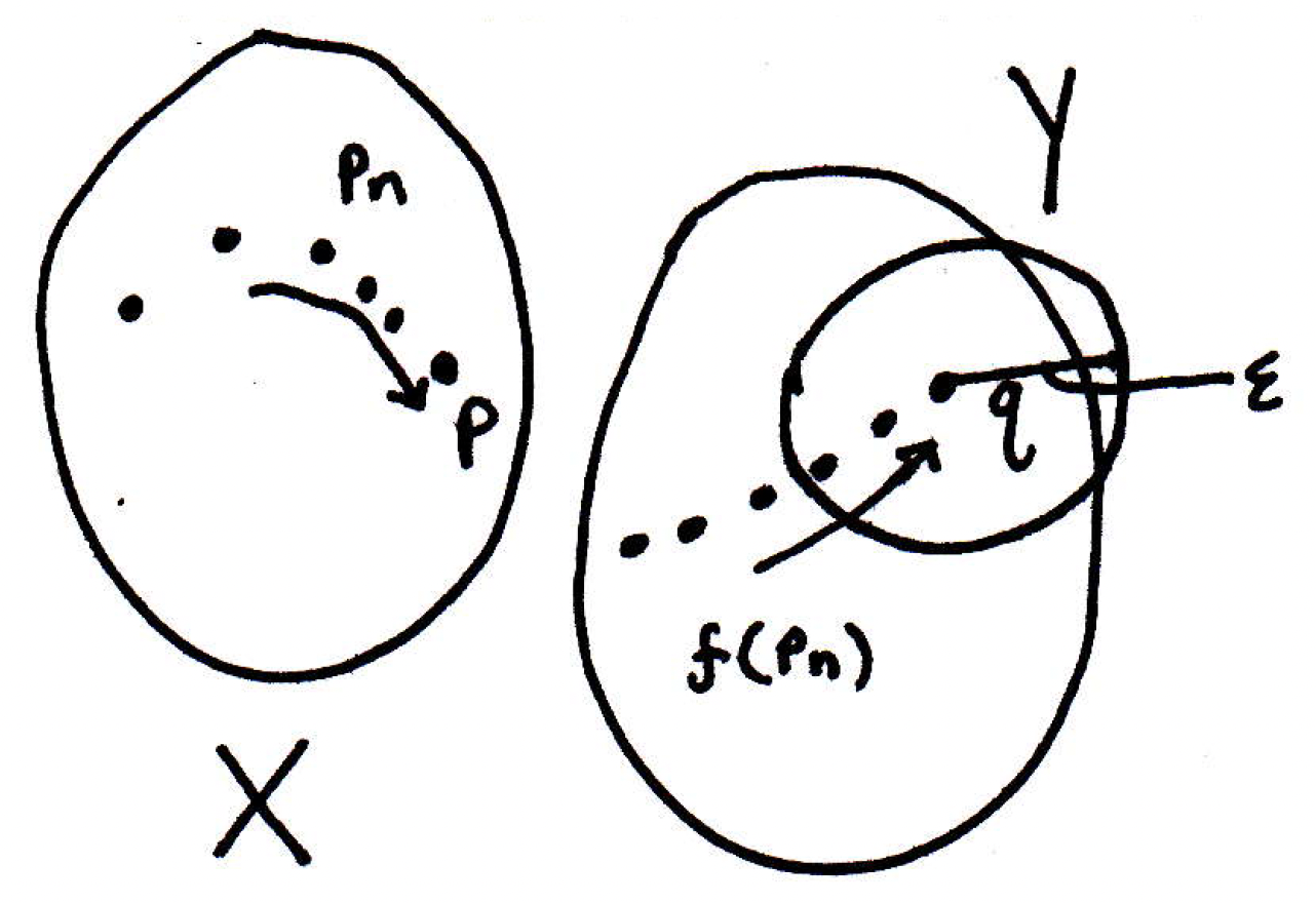
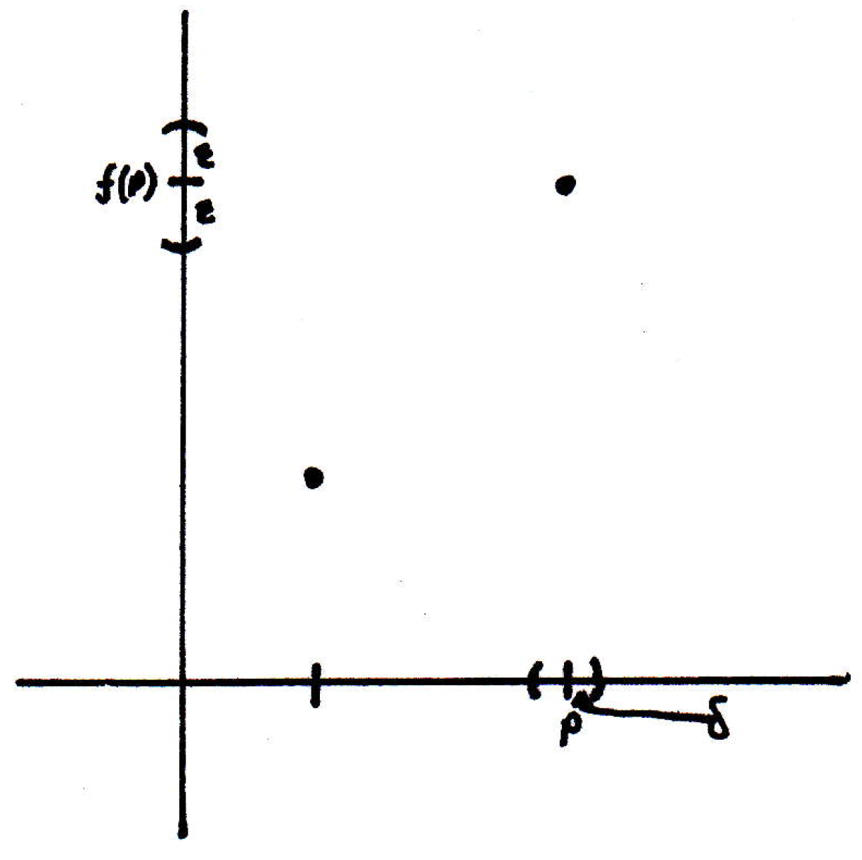
  To say "$f(x)\to q$ as $x\to p$" or "$\lim_{x\to p}f(x)=q$" means there exists $q\in Y$ such that what? We know from previous calculus work, perhaps, that we will have something like "for every $\epsilon>0$ there exists a $\delta>0$ such that \ldots." Here we will have the same basic idea, but we will be dealing with an $\epsilon$-ball around $q\in Y$ and a $\delta$-ball around $p\in X$ where it is the $\delta$-ball that is in $E$:

  

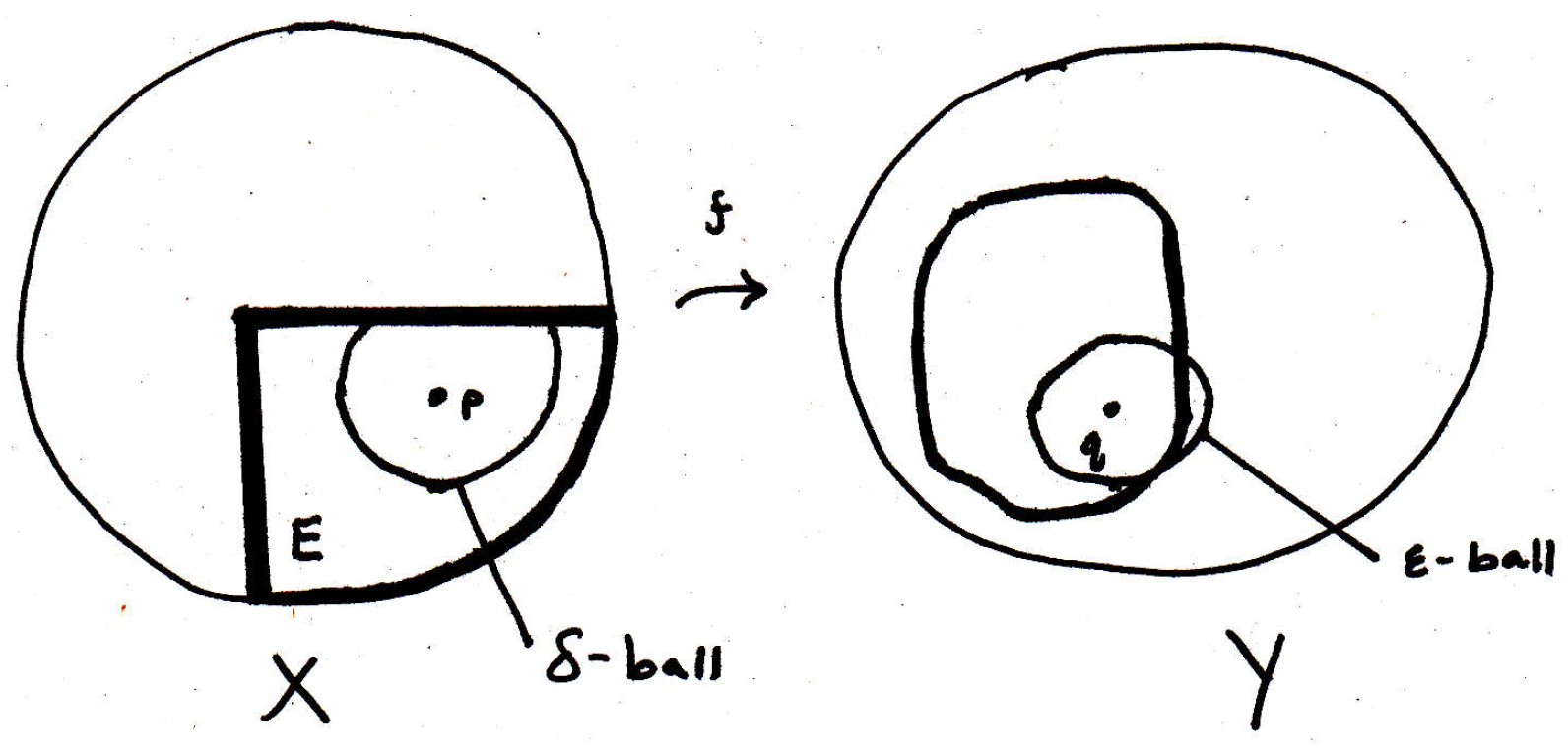
  Before, when we talked about sequences, we said that for any $\epsilon>0$ there is a point in the sequence beyond which you're close enough. Here we are going to say for $\epsilon>0$ there is a radius around $p$ for which if you're close in $E\subset X$ then you're close in $Y$. This radius we will call $\delta$, and this is a $\delta$-ball, and it is the $\delta$-ball that is contained in $E$.

  More precisely now, to say "$f(x)\to q$ as $x\to p$" or "$\lim_{x\to p}f(x)=q$" means there exists $q\in Y$ such that for all $\epsilon>0$ there exists $\delta>0$ such that for all $x\in E$, we have that $0<d_X(x,p)<\delta$ implies that $d_Y(f(x),q)<\epsilon$. We should note that $d_X$ and $d_Y$ denote the metrics on $X$ and $Y$, respectively. If we were dealing with the real numbers with the usual metric, then we'd be dealing with absolute values or normed differences. A curious thing about this definition is that we've said we're not looking at all things in the $\delta$-ball. There's one point that we're not allowing ourselves to look at, namely the point $x=p$. The condition $0<d_X(x,p)<\delta$ excludes the possibility of having $x=p$. So we're allowing the image of $p$ to do whatever the heck it wants to do.

• Limit (definition in [17]): Let $X$ and $Y$ be metric spaces; suppose $E\subset X$, $f$ maps $E$ into $Y$, and $p$ is a limit point of $E$. We write $f(x)\to q$ as $x\to p$, or

  $$\lim_{x\to p}f(x)=q$$

  if there is a point $q\in Y$ with the following property: For every $\epsilon>0$ there exists a $\delta>0$ such that

  $$d_Y(f(x),q)<\epsilon$$

  for all points $x\in E$ for which

  $$0<d_X(x,p)<\delta.$$

  The symbols $d_X$ and $d_Y$ refer to the distances in $X$ and $Y$, respectively.

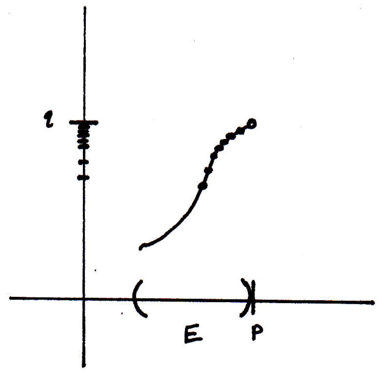
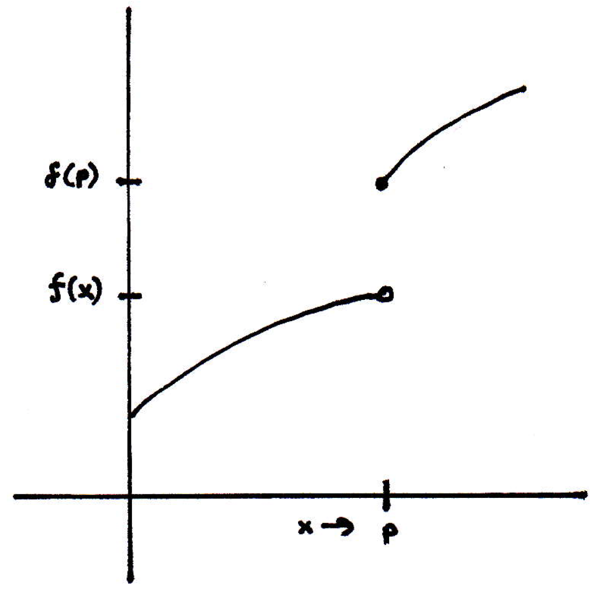
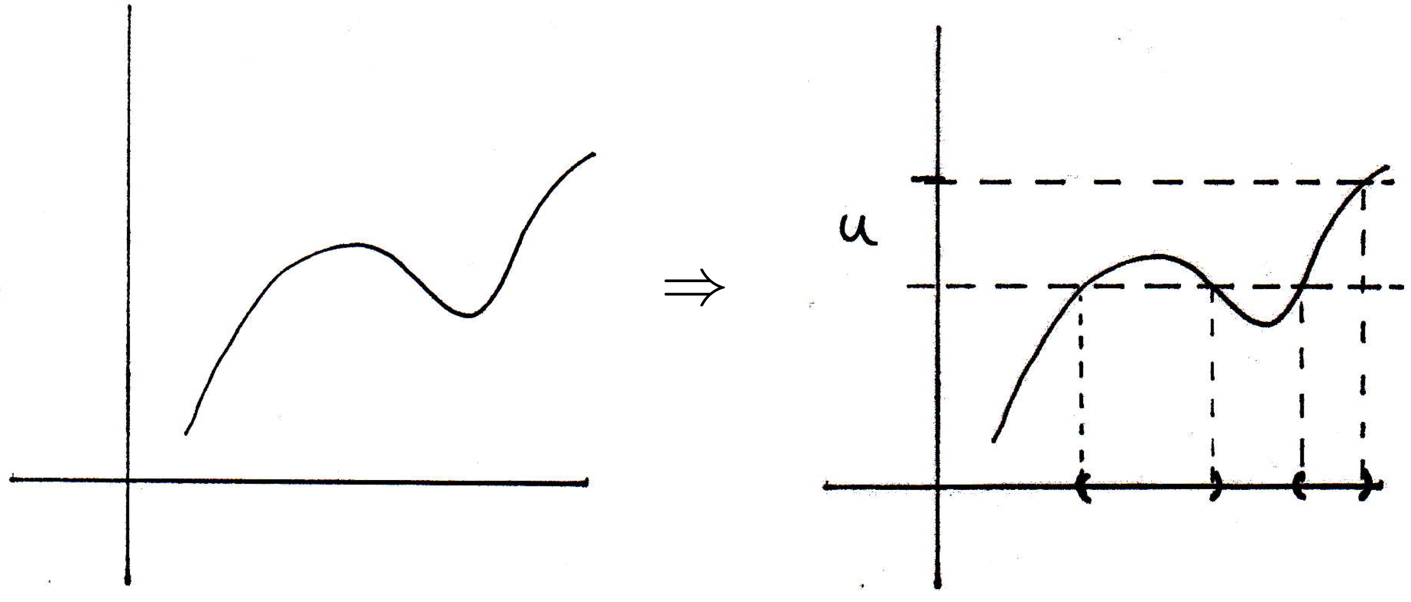
• Classic example: We don't care what's happening at $p$, only what's going on around it; that is, we should have $f(x)\to q$ as $x\to p$. And, of course, this should be from both directions in both cases:

  

  The above figure is the graph picture while

  

  is the mapping picture.

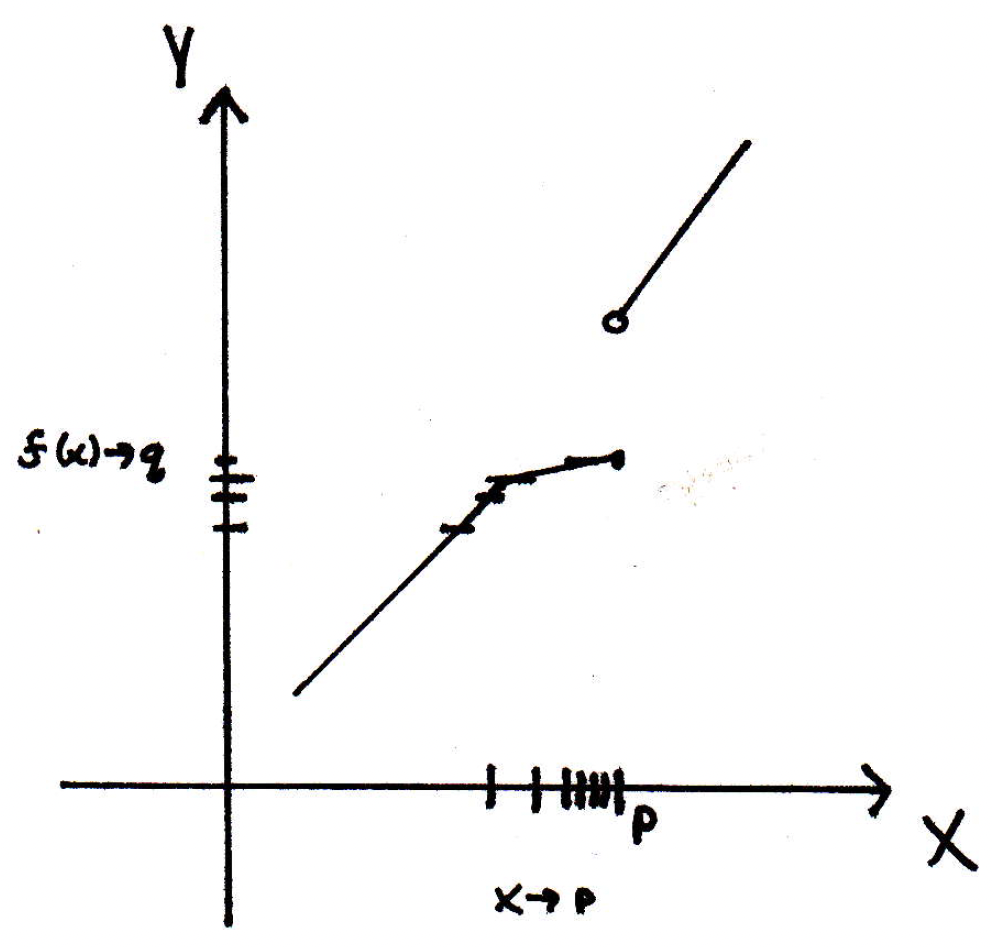
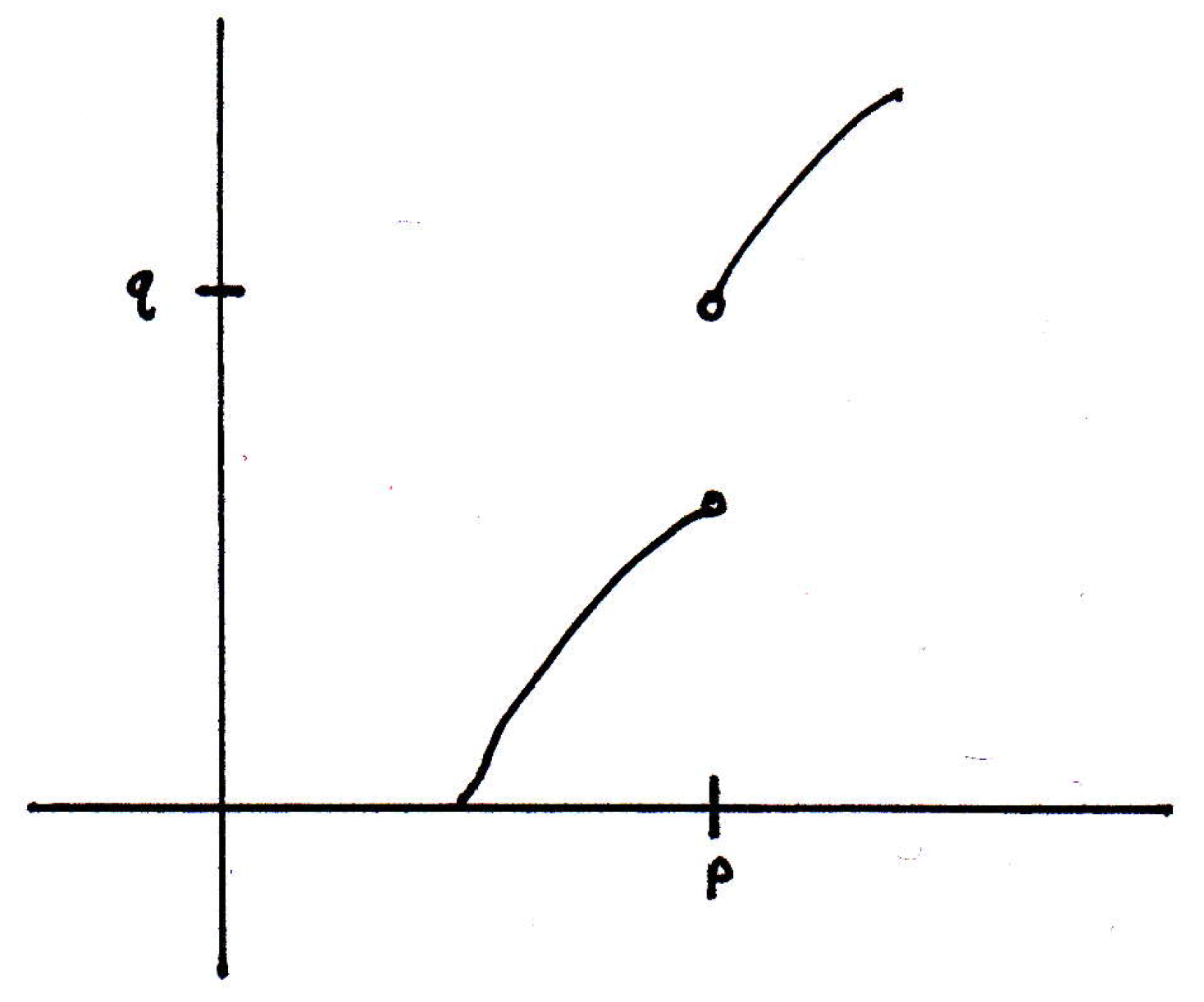
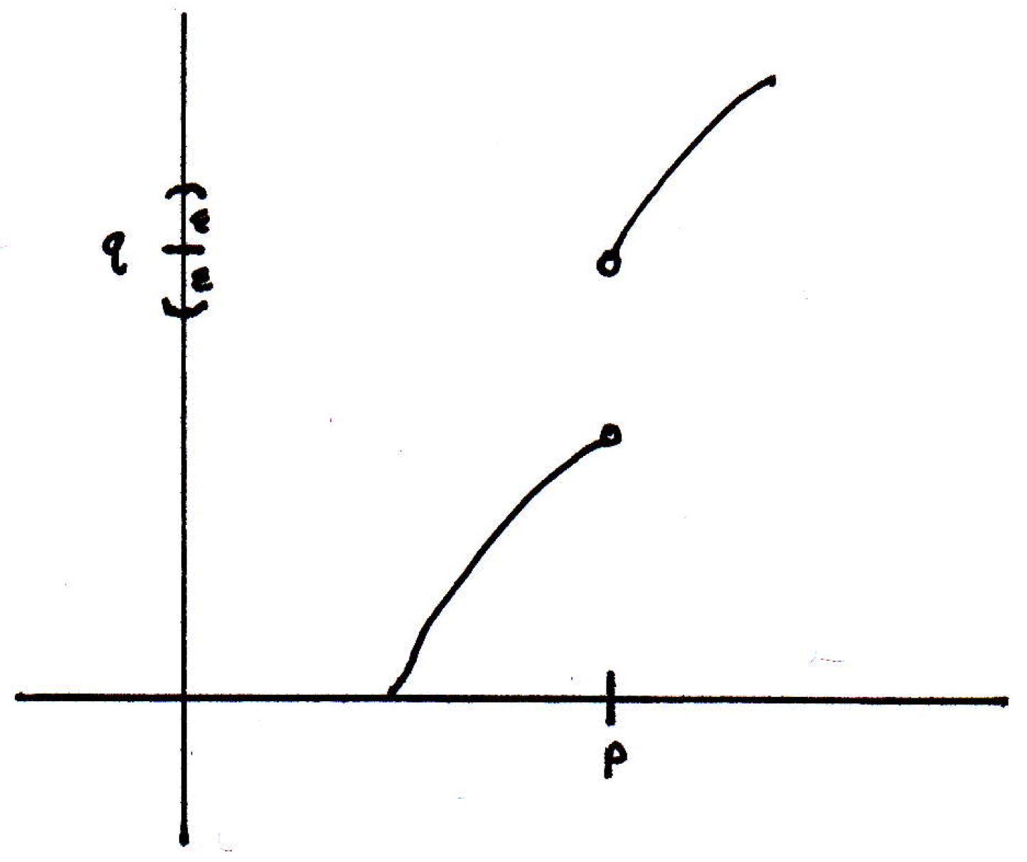
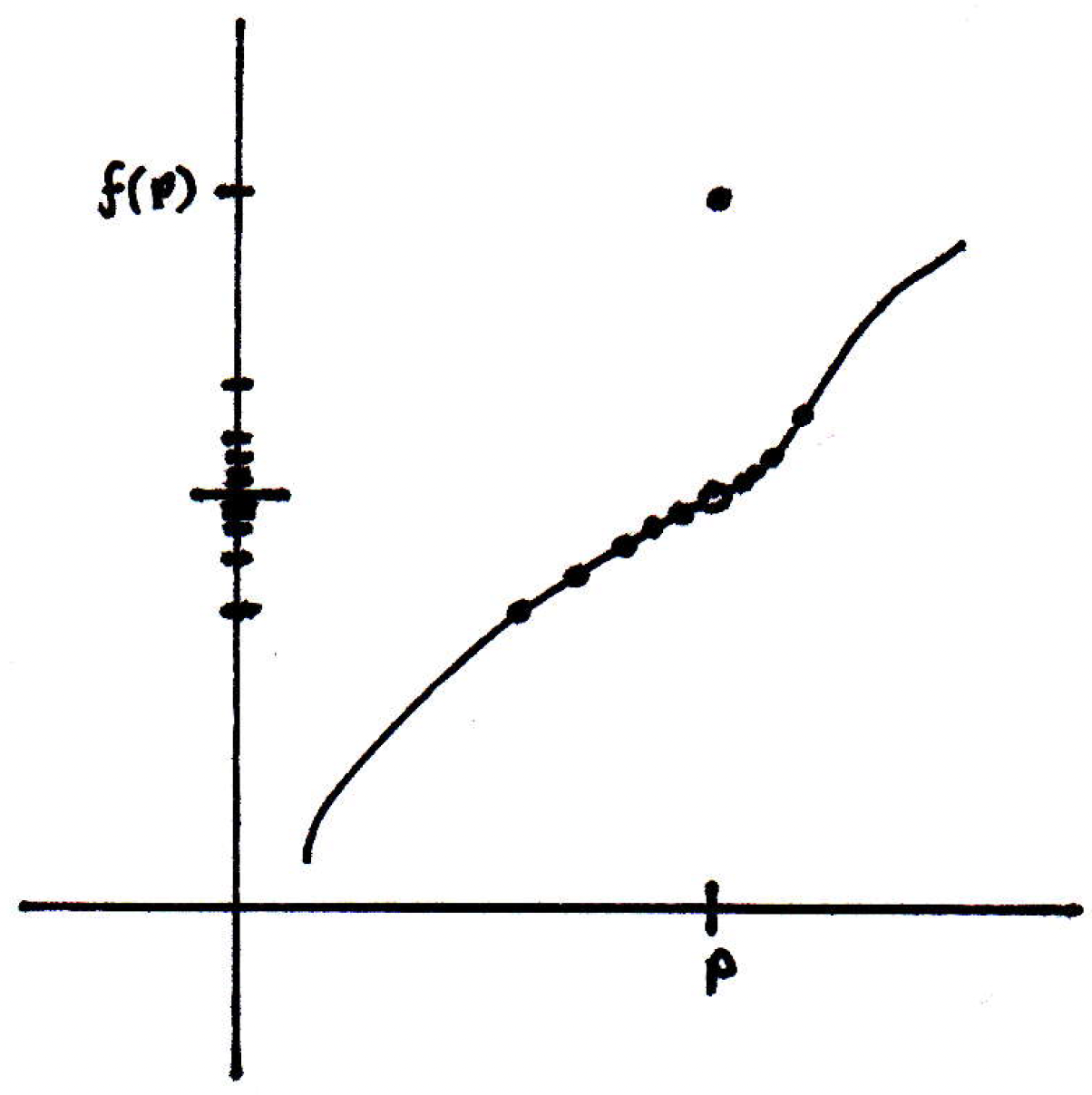
• Example: We will consider an example where the limit does not exist:

  

  If $x\to p$, then is there are $q$ for which if you're close enough to $p$ then you're close enough to $q$? No. We're converging to two different values from either direction. So there's no $q$ that will satisfy our definition.

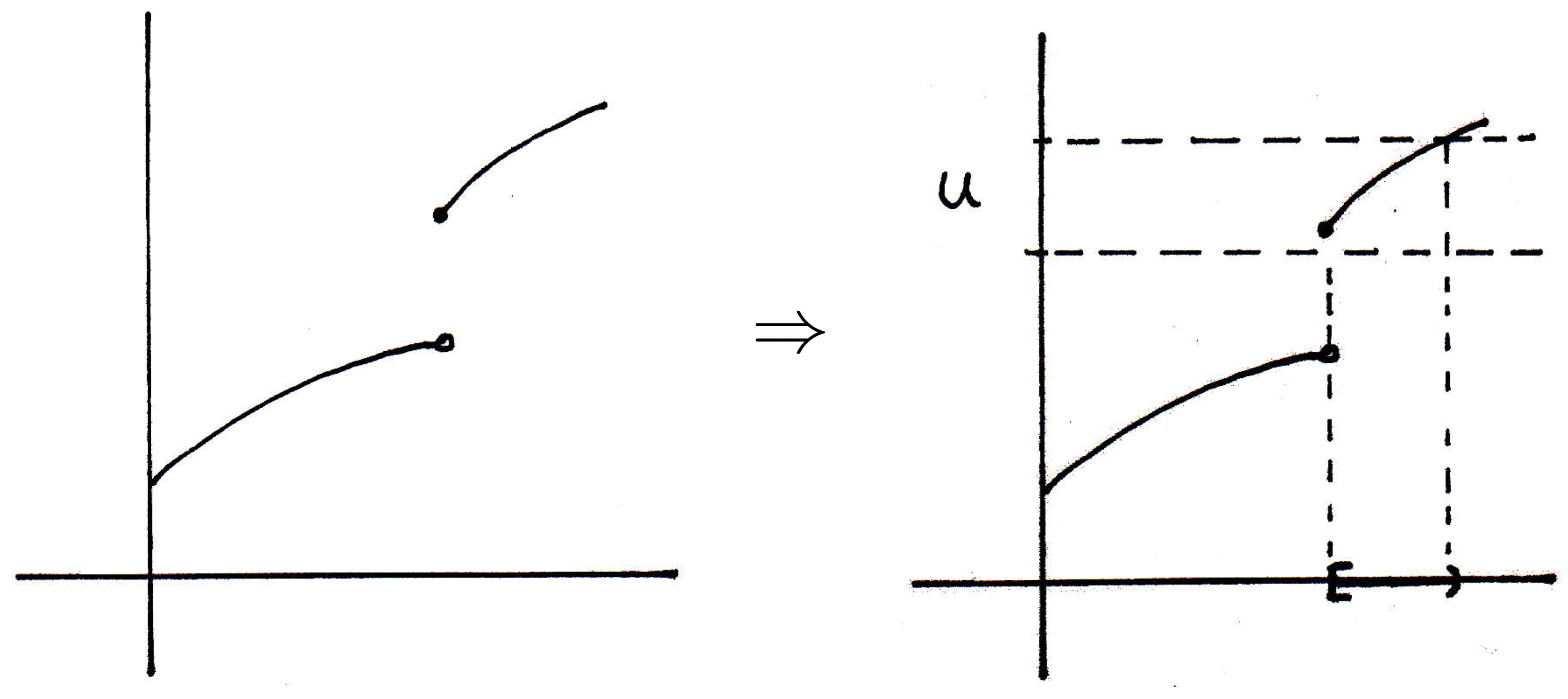
• Example: We don't require $E$ to contain $p$. So maybe $E$ is an open interval and $p$ is an endpoint. The only thing we require is that $p$ be a limit point of $E$. We want to be able to talk about a situation where maybe we have a function defined only on $E$, and it still makes sense to talk about convergence to some $q$:

  

  This is just pointing out all of the features of our limit definition.

• Remarks: So if you want to show convergence of a sequence, for every $\epsilon>0$ you have to find an $N$, an index. If you want to talk about convergence of a function, then for every $\epsilon>0$ you have to find a $\delta>0$. So your job to show convergence, given an $\epsilon>0$, is to find a $\delta>0$ that satisfies our definition.

• Remark about convergence: We used balls in the picture

  

  to talk about convergence, but you could think about convergence in terms of points that are getting closer and closer to $p$ and their images getting closer and closer to $q$. And so this brings up our first theorem about convergence of functions to limits of functions and that is it's equivalent to think of either way.

  So we could say $\lim_{x\to p}f(x)=q$ if and only if for all sequences $\{p_n\}\in E$, where $p_n\neq p$, and $p_n\to p$, we have $f(p_n)\to q$, where the latter part of this biconditional is the sequence characterization of function limits. The picture you should have is the following:

  

  Let's see why this equivalence is true. Let's prove this. How are we going to prove this? Just go to the definitions! This is how we prove anything. To summarize, here is the biconditional we are trying to prove:

  $$\lim_{x\to p}f(x)=q\iff (\forall \{p_n\}\in E)[(p_n\neq p)\land (p_n\to p)\implies f(p_n)\to q] \tag{(1)}$$

  It should be noted that the long proof that follows is succinctly given in [17].

• Proof of forward direction: Given $\epsilon>0$, our goal is to find an $N$ that works. That is, we want to find a point in the sequence beyond which all of the $f(p_n)$ terms are within $\epsilon$ of $q$:

  

  When will it be the case that all of the $f(p_n)$ will be in the $\epsilon$-ball? For the $\epsilon$-ball pictured in the figure above, there must exist a corresponding $\delta$-ball that satisfies the $\lim_{x\to p}f(x)=q$ definition:

  

  So what point of the sequence $f(p_n)$ should we look at? The images of the points that are in the $\delta$-ball. That's the whole idea of the proof right there. We cab now write this up more precisely.

  Given $\epsilon>0$, there exists $\delta>0$ such that $0<d_X(x,p)<\delta$ implies that $d_Y(f(x),q)<\epsilon$. For a given sequence $\{p_n\}$ that satisfies the conditions just listed, there exists $N$ such that $0<d_X(p_n,p)<\delta$. Thus, $n\geq N$ implies that $d_Y(f(p_n),q)<\epsilon$ due to the fact that $0<d_X(x,p)<\delta$ implies that $d_Y(f(x),q)<\epsilon$.

• Proof of backward direction: Suppose for all sequences $\{p_n\}$ in $E$, where $p_n\neq p$ and $p_n\to p$, we have $f(p_n)\to q$. We want to show that $\lim_{x\to p}f(x)=q$. How can we do this? Instead of proving this directly, it might be easier to prove the contrapositive. Let's try that. So suppose that $\lim_{x\to p}f(x)\neq q$. We need to show that there exists $\{p_n\}$ in$E$, where $p_n\neq p$ and $p_n\to p$, but $f(p_n)\not\to p$.

  To say that $\lim_{x\to p}f(x)=q$ is to say that

  $$(\forall\epsilon>0)(\exists\delta>0)(\forall x\in E)(0<d_X(x,p)<\delta\implies d_Y(f(x),q)<\epsilon).$$

  Thus, to say that $\lim_{x\to p}f(x)\neq q$ is to say that

  $$(\exists\epsilon>0)(\forall\delta>0)(\exists x\in E)(0<d_X(x,p)<\delta\land d_Y(f(x),q)\geq\epsilon).$$

  So, for the backward direction, assume that $\lim_{x\to p}f(x)\neq q$. That is, there exists $\epsilon>0$ such that for all $\delta>0$ there exists $x\in E$ such that $0<d_X(x,p)<\delta$ and $d_Y(f(x),q)\geq\epsilon$. What does this mean? It means there is an $\epsilon$-ball around $q$ such that no matter what $\delta$-ball you give me around $p$ then you can find a point in $E$ such that the distance between $p$ and $x$ is smaller than $\delta$ but the distance between their images is bigger than $\epsilon$.

  Can we use this information to construct a sequence that cannot converge to $q$? Consider the following picture:

  

  We can see an $\epsilon$-ball around $q$ which should work:

  

  We will have problems landing in that $\epsilon$-ball, particular as $x$ approaches $p$ from the left. Now, we don't care which $\delta$ is furnished. Suppose we have the following $\delta$-ball added to the picture:

  

  This $\delta$-ball is huge. We could make it very small. It doesn't matter. There will be a point $x$ in this $\delta$-ball which is close to $p$ but whose image is not $\epsilon$-close to $q$; that is, there will exists a point $x$ such that $0<d_X(x,p)<\delta$ but $d_Y(f(x),q)\geq\epsilon$:

  

  So let's use this to find a sequence. What sequence should we construct that will approach $p$ but whose image will not approach $q$? How about smaller and smaller $\delta$'s? We propose such a bad sequence. Use $\delta_n=\frac{1}{n}$ (these $\delta$'s get smaller and smaller) and choose $x_n$ according to

  $$(\exists\epsilon>0)(\forall\delta>0)(\exists x\in E)(0<d_X(x,p)<\delta\land d_Y(f(x),q)\geq\epsilon).$$

  Then $x_n\to p$, but $d_Y(f(x_n),q)\geq\epsilon$ by the condition above. Thus, $f(x_n)\not\to q$, thus concluding the proof.

• Recap about sequence characterization versus $\epsilon$-$\delta$ characterization: It doesn't matter if you want to talk about the sequence characterization or the $\epsilon$-$\delta$ characterization. They are two ways of saying the same thing. They are equivalent. The nice thing about the sequence characterization is that we've already proved many theorems about sequences. And they all carry over now to limits of functions. So, for instance, what do you know about sequences? Limits of sequences are unique. So limits of functions will be as well. Let's list a few things out concerning theorems we know about sequences that will carry over to functions (below we should note that $Y=\R$; otherwise, the results would not make sense unless $Y$ were a greater Euclidean space where you could prove similar theorems as well):

  • Limits are unique.
  • Limits of sums are sums of limits.
  • Limits of products are products of limits.

• Recap: So what do we have? We have described what it means for a function to have a limit. One of the places where this will be very important is to describe what it means for a function to be continuous.

Function continuity

How is continuity of functions defined, what are its uses, and what are some results?

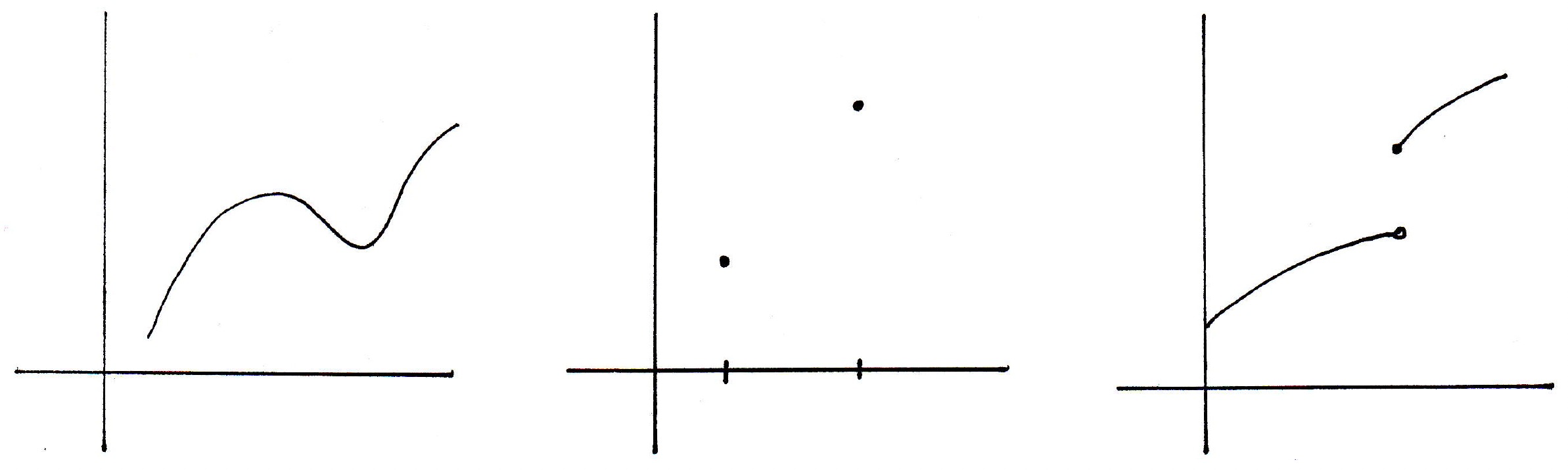
• Motivation: One of the most important concepts in analysis is the concept of a continuous function. This is a central concept of analysis, and we now have the machinery necessary to define what it means for a function to be continuous. First let's build some intuition. If I draw the graph of a function, what would you say is true about a continuous function? Is the following function continuous (where it's defined)?

  

  Is the following functions continuous where it's defined (just two points):

  

  Should the above function be called continuous? Maybe we take a look at a function that seems like it should clearly not be called continuous:

  

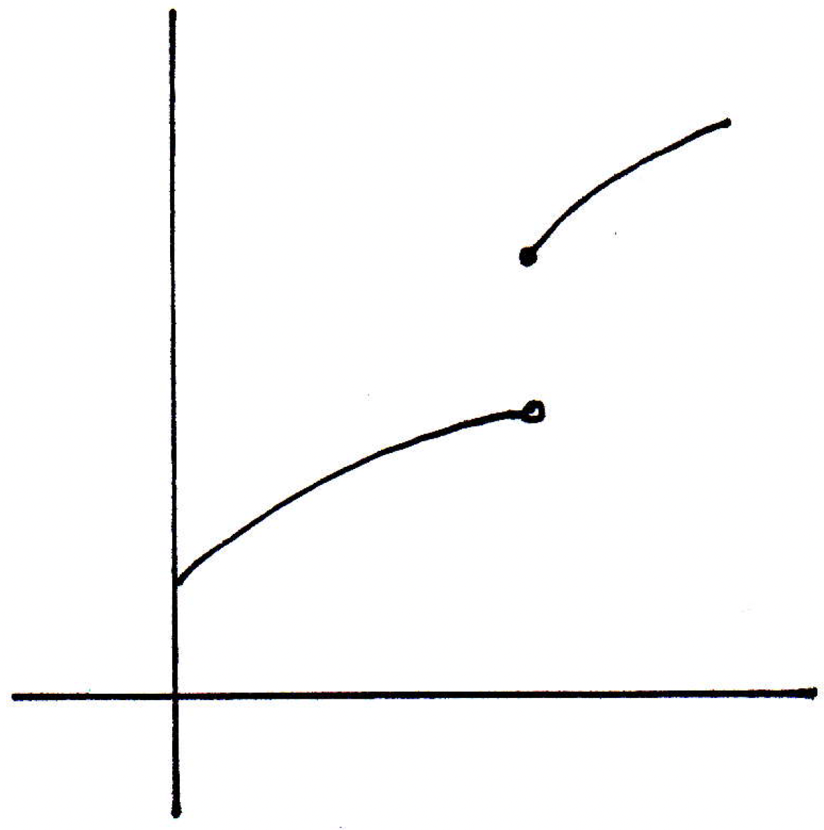
  Why would we say the above function is not continuous? The issue above is that as $x\to p$ we have $f(x)\not\to f(p)$ from the left:

  

  Even the following function is not continuous:

  

  The limit exists now, but we have the same problem as before. Here we have points converging to $p$ from both sides, and their images are converging too, but $f(p)$ is something completely different from what their images are converging to. So, what does it mean for a function to be continuous? It means the function value at every point is what its limit suggests. That's the intuitive way to think about it. Let's make a definition now.

• Continuity (definition from Su): Let $X$ and $Y$ be metric spaces, and now are going to consider some subset $E$ of $X$, but this time we will demand that $p$ be an element of the subset: $p\in E\subset X$. So let $X$ and $Y$ be metric spaces, where $p\in E\subset X$, and $f\colon E\to Y$. We say $f$ is continuous at $p$ if for every $\epsilon>0$ there exists $\delta>0$ such that for all $x\in E$ we have $d_X(x,p)<\delta$ implies that $d_Y(f(x),f(p))<\epsilon$. More concisely, given metric spaces $X$ and $Y$, where $p\in E\subset X$ and $f\colon E\to Y$, we say $f$ is continuous given the following:

  $$(\forall\epsilon>0)(\exists\delta>0)(\forall x\in E)(d_X(x,p)<\delta\implies d_Y(f(x),f(p))<\epsilon).$$

  Note that the limit condition $0<d_X(x,p)<\delta$ has been changed to $d_X(x,p)<\delta$ here because we may have $x=p$.

• Continuity (definition in [17]): Suppose $X$ and $Y$ are metric spaces, $E\subset X$, $p\in E$, and $f$ maps $E$ into $Y$. Then $f$ is said to be continuous at $p$ if for every $\epsilon>0$ there exists a $\delta>0$ such that

  $$d_Y(f(x),f(p))<\epsilon$$

  for all points $x\in E$ for which $d_X(x,p)<\delta$. If $f$ is continuous at every point of $E$, then $f$ is said to be continuous on $E$.

• Theorem (see [17]): If $p$ is a limit point of $E$, then $f$ continuous at $p$ then this is equivalent to $\lim_{x\to p}f(x)=f(p)$. Now, recall the sequence characterization in (1). So here's really what we are saying with this theorem: Suppose we look at the sequence characterization. What we're saying with

  $$\lim_{x\to p}f(x)=f(p)$$

  is that if you take a sequence converging to $p$, then the limit of $f$ of the sequence is $f$ of the limit of the sequence. That is, if $\{x_n\}$ is a convergent sequence, then $f$ continuous is equivalent to say $\lim_{n\to\infty}f(x_n)=f(\lim_{n\to\infty} x_n)$. In other words, for continuous functions, you can switch continuous functions and limits. It doesn't matter which order you apply them. That's a very important property. The limiting operation and the function operation commute when dealing with continuous functions.

• Revisitation: Let's revisit an earlier figure:

  

  Is this function continuous? Well, there are only two points for which to check continuity. It doesn't matter. Let's just consider the point on the right:

  

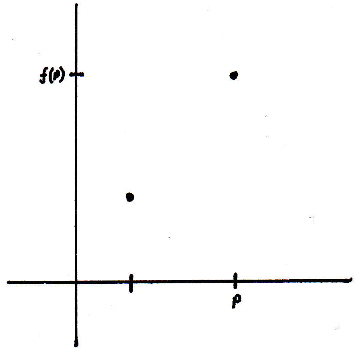
  Is it true that $f$ is continuous at $p$? Is it true that for every $\epsilon$ you name there is a $\delta$ around which as long as you're within some $\delta$ of $p$ then you're within some $\epsilon$ of $f(p)$. So let's consider any $\epsilon$-ball around $f(p)$, say the following:

  

  Can we find a $\delta$-ball around $p$ so that everything in the $\delta$-ball that is in $E$ also lands in the $\epsilon$-ball around $f(p)$? Sure:

  

  So is this function continuous? Yes! The $\delta$-ball has nothing else in it other than one point. This is a rather interesting example. This example actually illustrates something that holds in general: If you take a function from a discrete metric space to any other metric space, then your function will automatically be continuous, and this should make some intuitive sense because all of the points are separated in a discrete metric space. So you vacuously cannot approach points and the conditions for continuity hold in a rather trivial way.

• Corollary for continuous functions: Sums, differences, products, and quotients for continuous functions are continuous as well, where it is clear our metric space $Y=\R$ in this case and also that $g\neq0$ when dealing with a quotient of the form $\frac{f}{g}$. This corollary is due to the "limit laws" we established as well as the limit point theorem we proved above.

• Corollary (see [17]): Suppose we have vector-valued functions and we map a metric space into a vector. So let $f,g\colon X\to\R^k$ such that $\bm{f}=(f_1,\ldots,f_k)$ and $\bm{g}=(g_1,\ldots,g_k)$. Then we have the following:

  1. $\bm{f}$ is continuous if and only if each $f_i$ are continuous

  Proof. Why is this rule true? We just have to do some bounding. In one case we are trying to make the distance between two points small, namely the distance between $f(x)$ and $f(p)$. We want to make that distance small in one case. In the other case, we are trying to make the distance between $f_i(x)$ and $f_i(p)$ small. So if I have that one is small, can I show that the other is small? Is $|f_i(x)-f_i(p)|$ somehow related to $||f(x)-f(y)||$? Yes, we also have components we are dealing with when looking at $||f(x)-f(y))||$. We always have the bound

  $$|f_i(x)-f_i(p)|\leq ||f(x)-f(y)||.$$

  We use this fact. If we make $||f(x)-f(y)||$ smaller than $\epsilon$ for some $\delta$, then $|f_i(x)-f_i(p)|$ will automatically be smaller than $\epsilon$ for the same $\delta$.

  Now, what if we need to make $||f(x)-f(y)||$ small and we know $|f_i(x)-f_i(p)|$ is always small? Well, if we know all $|f_i(x)-f_i(p)|$ are small, then isn't $||f(x)-f(y)||$ just some combination of all of these; that is, $||f(x)-f(y)||=\sqrt{\sum_{i=1}^k|f_i(x)-f_i(p)|^2}$?

  2. $\bm{f}+\bm{g}$, $\bm{f}\cdot\bm{g}$ are continuous

  Proof. Use components from the first part. It follows from that.

• Recap: What do we know so far? Well, we know what it means for a function to be continuous. We have two different characterizations of continuity (functions and sequences, one involving $\epsilon$'s and $\delta$'s and the other involving $\epsilon$'s and a choice of $N$). It turns out there is another characterization of continuity, and this one is, perhaps, not at all obvious.

• Another characterization of continuity: There is a characterization of continuity in terms of open sets.

• Continuity in terms of open sets (theorem; see [17]): The function $f\colon X\to Y$ is continuous if and only if for all open sets $U$ in $Y$ we have $f^{-1}(U)$ is open in $X$. What does this have to do with continuity? What are we saying? Let's draw a picture:

  

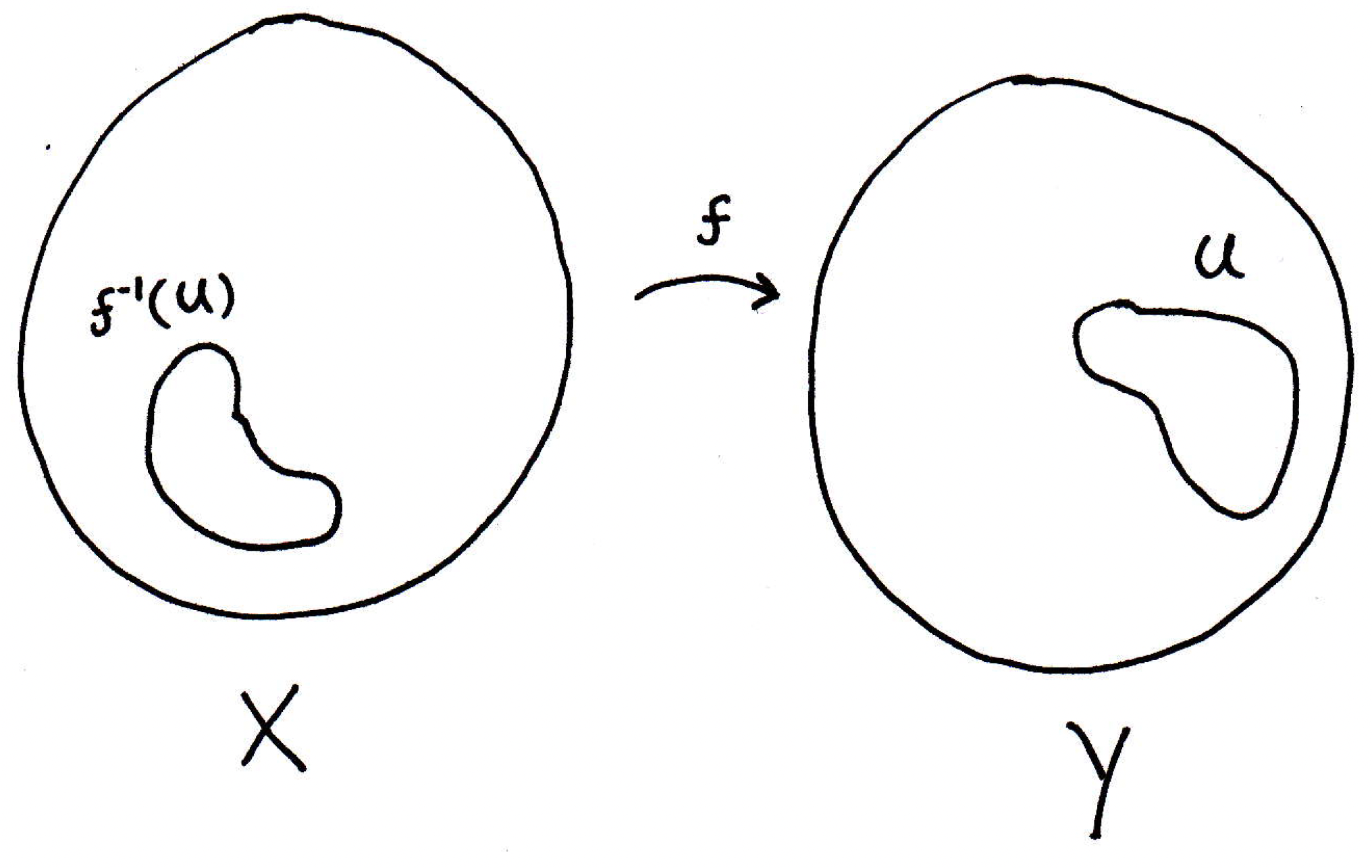
  The claim is that $f$ will be continuous if for any open set $U$ we pick in $Y$, then it will have an inverse image $f^{-1}(U)$ in $X$ that is also open. Similarly, if it is the case that for every open set $U$ in $Y$ that $f^{-1}(U)$ is open in $X$, then $f$ is continuous. Why might this be true? Let's recall some of the functions we dealt with earlier:

  

  Let's deal with each of these functions separately, and see how the theorem is true or false depending on the function we are dealing with. For the first function, we said it's continuous. If we take an open set $U$, then will its inverse image be open? Let's see:

  

  What does the above picture mean? The open set $U$ represents everything that falls in the ribbon, and $f^{-1}(U)$ is composed of the two intervals mapped to below the ribbon, where note these intervals are open (and recall the union of countably or uncountably many open sets is open). If we labeled the intervals $I_1$ and $I_2$, then $f^{U}=I_1\cup I_2$. Since $I_1$ and $I_2$ are both open sets, then it follows that their union, and hence $f^{-1}(U)$, is also open. What about the second function? We would have the following:

  

  Here, the set $f^{-1}(U)$ is not open. It's half-open, and that should make sense because we knew from the start that $f$ was not continuous, and this picture supports our theorem; that is, we claim the inverse image, $f^{-1}(U)$ is not open because $f$ is not continuous. What about the last picture? We'd have the following:

  

  Is the point open in the two-point set? Discrete metric. Yes. So it works.

• Proof idea: The definition of continuity just given, in terms of open sets and the like, is probably the most useful or best definition of continuity. Why?

  1. If you're a topologist, then you don't like referring to metrics necessarily. This is actually a definition of continuity that will hold for general topological spaces. You don't have to refer to distances or metrics. That's probably the best reason why it's a good definition. It's the most elegant in some sense. It just refers to the topology of the real line. You're only referring to what you consider to be open sets.

  2. It's also a question that often appears, in some way, on the Math GRE if you're going to graduate school for math. There's usually some question that tests your understanding of this definition.

  It would be informative to think of how you can prove the theorem under consideration using the $\epsilon$-$\delta$ definition.

• End note: If we replaced the "open set" conditions in our theorem with "closed set" then that's another definition of continuity. The inverse image of closed sets is closed. Why is that? By complements or "complementation." There are a number of different equivalent definitions of continuity.